Python for Algorithmic Trading: Essential Libraries
Python's hold on algorithmic trading comes from its libraries, and the useful way to learn them is by the stage of the workflow each one serves: getting data in, computing indicators, testing statistics, backtesting a rule, fitting a model, and drawing the result. This guide maps the essential libraries to those stages, explains what each does well and where it stops, notes which projects are actively maintained, and shows runnable code for the parts that matter most, with no API keys and no invented benchmarks. It closes with where Quant Charts fits: the same rule you would backtest in Python can be described to Quant, our coding agent, which writes it in Pine Script and runs the Backtest Summary on the chart before you commit to a notebook.
Key points:
- pandas and NumPy are the foundation; everything else consumes or produces their arrays and frames. Polars, DuckDB and PyArrow join when data outgrows memory or patience.
- Indicators are easy; frameworks are a choice. TA-Lib and pandas-ta compute the standard set, but writing a moving average yourself is a better first lesson.
- Pick a backtester for the job. vectorbt for parameter sweeps, Backtesting.py for readable event-driven rules, Backtrader and Zipline for mature ecosystems, LEAN when you want a full engine.
- Machine learning needs time-aware validation. scikit-learn's TimeSeriesSplit, not a random split, and features that were knowable at the time.
The Library Map
| Stage | Libraries | What they do | Notes |
|---|---|---|---|
| Data access | yfinance; broker and exchange SDKs | Download historical bars and reference data | yfinance is community-maintained and fine for research; production systems use a paid feed |
| Data handling | pandas, NumPy | Time-series frames, alignment, resampling, vectorised arithmetic | The common currency of the ecosystem |
| Scale | Polars, DuckDB, PyArrow | Columnar frames, SQL over Parquet, zero-copy interchange | For tick data or many years of minute bars |
| Indicators | TA-Lib (ta-lib-python), pandas-ta | Standard technical indicators | TA-Lib needs the C library installed; pandas-ta is pure Python |
| Statistics | statsmodels, SciPy | Regression, stationarity and cointegration tests, distributions, optimisation | Where strategy ideas are checked before they become rules |
| Backtesting | vectorbt, Backtesting.py, Backtrader, Zipline (zipline-reloaded), LEAN | Simulate rules over history with costs and fills | Compared below |
| Machine learning | scikit-learn, PyTorch, TensorFlow | Classification, regression, sequence models | Validation discipline matters more than model choice |
| Visualisation | Matplotlib, Plotly | Static figures and interactive charts | Matplotlib for notebooks and papers; Plotly for dashboards |
Data: pandas and NumPy
pandas gives you the DataFrame, a table indexed by time, with the operations a trader needs built in: resampling bars to a coarser timeframe, aligning series with different calendars, rolling windows, shifts and joins. NumPy underneath does the arithmetic in compiled code, which is why a vectorised expression over a million rows finishes in milliseconds while the same logic in a Python loop takes minutes. The snippet below loads adjusted daily bars, computes returns and a rolling volatility, and resamples to weekly bars, which covers most of what research code does with data.
import numpy as np
import pandas as pd
import yfinance as yf

bars = yf.download("SPY", start="2015-01-01", end="2025-01-01",
                   auto_adjust=True, progress=False)
bars.columns = [c[0] if isinstance(c, tuple) else c for c in bars.columns]   # flatten MultiIndex

close = bars["Close"]
returns = close.pct_change()
vol_20 = returns.rolling(20).std() * np.sqrt(252)          # annualised 20-day volatility

weekly = bars.resample("W-FRI").agg({"Open": "first", "High": "max",
                                     "Low": "min", "Close": "last", "Volume": "sum"})
print(weekly.tail(3))
Two habits pay off immediately. Keep prices adjusted for splits and dividends, or returns will show phantom crashes. And never use a value in a calculation for a bar before it was known; pandas makes lookahead easy to introduce with a misplaced shift, and the fix is to reason about every rolling window and shift in terms of which bar it was available on.
When Data Outgrows pandas
Minute bars for a few hundred symbols, or any tick data, stop fitting comfortably in memory. Polars offers a columnar DataFrame with lazy evaluation and multi-threaded execution; DuckDB queries Parquet and CSV files with SQL directly from Python, so the aggregation happens in the database engine and only the result becomes a frame; PyArrow is the interchange format both use, and Parquet is the file format to store bars in. Our SQL for trading guide covers the database side, and none of it is necessary until pandas becomes the bottleneck.
Indicators: TA-Lib, pandas-ta, or Your Own
TA-Lib is the long-standing C library of technical indicators, exposed to Python through the ta-lib-python wrapper; it is fast and its calculations are the reference implementations most platforms match, but installing the C library is the classic first hurdle. pandas-ta is pure Python, installs with pip, and covers a similar range with a pandas-native interface. Both are convenient. Neither is necessary for the common indicators, and writing a few yourself is the fastest way to understand what a rolling window is doing on every bar.
def sma(series, length):
    return series.rolling(length).mean()

def rsi(series, length=14):
    """Wilder's RSI: exponentially smoothed average gains over average losses."""
    change = series.diff()
    gain = change.clip(lower=0)
    loss = -change.clip(upper=0)
    avg_gain = gain.ewm(alpha=1 / length, adjust=False, min_periods=length).mean()
    avg_loss = loss.ewm(alpha=1 / length, adjust=False, min_periods=length).mean()
    rs = avg_gain / avg_loss
    return 100 - 100 / (1 + rs)

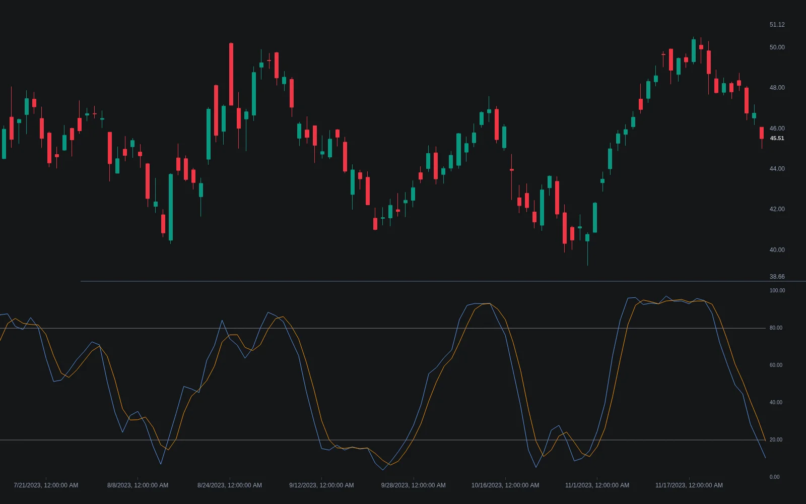
def stochastic(high, low, close, k_length=14, k_smooth=3, d_smooth=3):
    lowest = low.rolling(k_length).min()
    highest = high.rolling(k_length).max()
    raw_k = 100 * (close - lowest) / (highest - lowest)
    k = raw_k.rolling(k_smooth).mean()
    d = k.rolling(d_smooth).mean()
    return k, d

bars["sma_20"] = sma(close, 20)
bars["rsi_14"] = rsi(close, 14)
bars["stoch_k"], bars["stoch_d"] = stochastic(bars["High"], bars["Low"], close)
The RSI here uses Wilder's smoothing, which is what charting platforms plot; a version built on simple averages gives different numbers, and the difference matters when you compare a backtest with a chart. When a library and your own code disagree, that is usually why.
Statistics: statsmodels and SciPy
Before a pattern becomes a rule it should survive a statistical question, and statsmodels is where those questions are asked in Python: ordinary least squares for hedge ratios and factor exposures, the augmented Dickey-Fuller and KPSS tests for stationarity, the Engle-Granger test for cointegration, ARIMA and GARCH-style models for series and volatility. SciPy supplies the distributions, the optimisers used for portfolio weights and the numerical routines under everything else. Our mean reversion guide shows the stationarity tests in use, and risk parity with Python uses SciPy's optimiser to solve for portfolio weights.
Backtesting Frameworks
A backtester turns a rule into simulated trades with fills, costs and a report. The Python options differ mainly in how they iterate and how much they assume, and the right one depends on whether you are sweeping parameters or simulating a realistic order flow.
| Framework | Model | Strength | Consider |
|---|---|---|---|
| vectorbt | Vectorised over NumPy arrays | Very fast; thousands of parameter combinations in one run; rich portfolio statistics | Path-dependent rules are harder to express; the open-source core and a commercial edition differ |
| Backtesting.py | Event-driven, one Strategy class | Small, readable API; built-in optimiser and interactive plots | Single-instrument focus; simple fill model |
| Backtrader | Event-driven, feature-rich | Mature: brokers, sizers, analyzers, multi-data, live-trading adapters | Development has slowed; check recent activity before building on it |
| Zipline (zipline-reloaded) | Event-driven with data bundles and a Pipeline API | Institutional-style design for cross-sectional strategies; maintained as zipline-reloaded | Data bundle set-up is heavier than the alternatives |
| LEAN (QuantConnect) | Full engine in C# with a Python API | Multi-asset, realistic modelling, same code runs in backtest and live | Heaviest to run locally; usually paired with the hosted platform |
Backtesting.py is the quickest way to see the event-driven shape that every framework shares: a class with an init method that computes indicators and a next method that is called once per bar and places orders. The example trades a moving average crossover with a percentage commission; fills happen on the next bar's open by default, which is the honest choice.
from backtesting import Backtest, Strategy
from backtesting.lib import crossover

class SmaCross(Strategy):
    fast = 10
    slow = 30

    def init(self):
        price = self.data.Close
        self.ma_fast = self.I(sma, pd.Series(price), self.fast)
        self.ma_slow = self.I(sma, pd.Series(price), self.slow)

    def next(self):
        if crossover(self.ma_fast, self.ma_slow):
            self.buy()
        elif crossover(self.ma_slow, self.ma_fast):
            self.position.close()

bt = Backtest(bars[["Open", "High", "Low", "Close", "Volume"]], SmaCross,
              cash=10_000, commission=0.001, exclusive_orders=True)
stats = bt.run()
print(stats[["# Trades", "Return [%]", "Max. Drawdown [%]", "Sharpe Ratio"]])
Whatever the framework, the discipline is identical: decide on the close and fill on the next bar, charge a cost on every fill, hold out a period the parameters never saw, and treat a small trade count as no evidence. The backtesting engine in Python guide builds the machinery from scratch for readers who want to understand what these libraries do internally, and backtesting traps lists the mistakes they cannot prevent.
Machine Learning: scikit-learn, PyTorch, TensorFlow
scikit-learn covers classical machine learning, random forests, gradient boosting, logistic regression, support vector machines, with a consistent interface and, critically for trading, cross-validation tools that respect time. The mistake that ruins most trading models is not the algorithm but the validation: a random train-test split lets the model see the future, and features computed with information from after the bar leak the answer into the question. TimeSeriesSplit trains on the past and tests on what follows, and every feature should be something you could have computed at the close of the bar it is attached to.
from sklearn.ensemble import GradientBoostingClassifier
from sklearn.model_selection import TimeSeriesSplit
from sklearn.metrics import accuracy_score

features = pd.DataFrame({
    "ret_1": returns,
    "ret_5": close.pct_change(5),
    "rsi_14": bars["rsi_14"],
    "vol_20": vol_20,
    "dist_sma": close / bars["sma_20"] - 1,
}).dropna()

# Label: does the next bar close higher? Known only after the fact, so it is shifted back one bar.
label = (close.shift(-1) > close).astype(int).loc[features.index]

scores = []
for train_idx, test_idx in TimeSeriesSplit(n_splits=5).split(features):
    model = GradientBoostingClassifier(n_estimators=200, max_depth=3, random_state=0)
    model.fit(features.iloc[train_idx], label.iloc[train_idx])
    preds = model.predict(features.iloc[test_idx])
    scores.append(accuracy_score(label.iloc[test_idx], preds))

print("fold accuracies:", [round(s, 3) for s in scores])   # compare with the base rate of up days
Read the accuracies against the base rate, the fraction of up days in the test folds, not against fifty percent; a model that matches the base rate has learned nothing. PyTorch and TensorFlow add deep learning, sequence models and GPU training, which are justified for large alternative datasets and text but rarely for a handful of price-derived features, where they overfit faster than they learn. Whatever the model, its output is a signal to be backtested with costs like any other, not a strategy in itself.
Visualisation: Matplotlib and Plotly
Matplotlib draws the static figures that belong in a notebook or a report: equity curves, drawdown plots, return distributions, indicator overlays, all with fine control over every element and direct plotting from pandas. Plotly produces interactive charts that zoom, pan and show values on hover, and it is the natural choice for a dashboard or for exploring a long series. Use both: Matplotlib to check and document, Plotly to explore and share. Whichever you use, plot equity on a log scale, so that a strategy's growth rate is readable across the whole history rather than dominated by its final years.
A Minimal Environment
python -m venv .venv && source .venv/bin/activate
pip install pandas numpy scipy statsmodels yfinance matplotlib plotly scikit-learn backtesting
# optional, as the work demands:
pip install pandas-ta vectorbt polars duckdb pyarrow
Pin versions in a requirements file once a project produces results you care about; a backtest that cannot be reproduced next month because a library changed its defaults is a common and avoidable loss.
Pitfalls the Libraries Will Not Catch
| Pitfall | How it appears | Fix |
|---|---|---|
| Lookahead | A rolling value or label that includes information from after the bar | Reason about availability per bar; shift labels back, never features forward |
| Unadjusted prices | Splits look like crashes; dividends inflate drawdowns | Use adjusted series, or keep raw prices with a corporate-actions table |
| Random validation splits | A model that scores well and fails live | TimeSeriesSplit or a walk-forward loop |
| Indicator mismatch | Backtest signals differ from the chart | Match the smoothing method; Wilder versus simple averages is the usual culprit |
| Costless fills | High-turnover rules look profitable | Commission and slippage on every fill; re-run at double |
| Unmaintained dependencies | Install failures and silent behaviour changes | Check release activity; pin versions; prefer maintained forks such as zipline-reloaded |
| Notebook state | Results that depend on cell execution order | Restart and run all before trusting a number; move logic into modules |
Where Quant Charts Fits
Most of the work above exists to answer one question: does this rule survive an honest test? Quant Charts answers it faster for any rule that lives on a chart. Describe the strategy to Quant, the crossover from the Backtesting.py example, a stochastic exit, a volatility filter, and Quant writes it in Pine Script and plots it on the active chart. Open Code to read the logic, click Run, and the Backtest Summary reports net profit, trade count, win rate, maximum drawdown and profit factor with commission and slippage set in the strategy properties. A rule that fails there does not need a notebook; a rule that passes arrives in Python with a specification and a benchmark to match. The Making Strategies with Quant guide shows the workflow, and Library indicators such as the Stochastic load in a click, with their Pine Script source published for anyone who wants to compare against the pandas version.
For Python developers there is a second bridge: PineTS, LuxAlgo's open-source runtime for Pine Script®, runs Pine logic outside TradingView, so an indicator written for the chart can be reproduced in a service and compared with its Python twin. One boundary: the LuxAlgo platform does not place orders for you, so execution remains your own code, for example through our open-source Trade Relay and Broker SDK.
Conclusion
The Python trading stack is deep, but it is not mysterious: pandas and NumPy hold the data, a handful of indicator and statistics libraries transform it, a backtester chosen for the job simulates the rule, scikit-learn and its heavier cousins fit models when there is enough data to justify them, and Matplotlib and Plotly show the result. The libraries are excellent and none of them will stop you from looking into the future, ignoring costs or trusting a model that learned the base rate. Those habits are yours to build. Build them on Quant Charts first, where Quant writes the Pine Script and the Backtest Summary judges the rule, and bring to Python the rules that have earned the effort.
Key Takeaways
- Learn by stage. Data, indicators, statistics, backtesting, models, charts; each has two or three libraries worth knowing.
- pandas and NumPy first. Adjusted prices, careful shifts, vectorised arithmetic; Polars and DuckDB when the data outgrows them.
- Choose the backtester for the job. vectorbt to sweep, Backtesting.py to read, Backtrader or Zipline for depth, LEAN for a full engine; all with next-bar fills and costs.
- Validate in time order. TimeSeriesSplit and knowable features; compare against the base rate.
- Prototype on Quant Charts. Quant writes the Pine Script, Code shows it, Run backtests it; Python takes over for what passes.
FAQs
Which Python libraries do I need to start algorithmic trading?
pandas and NumPy for data, yfinance for research downloads, statsmodels and SciPy for statistics, one backtesting framework such as Backtesting.py or vectorbt, scikit-learn if you plan to fit models, and Matplotlib or Plotly for charts. TA-Lib or pandas-ta are convenient for indicators but optional; writing a moving average and an RSI yourself is a better first exercise.
Should I use TA-Lib or pandas-ta?
TA-Lib is the reference C implementation with a Python wrapper; it is fast and matches most platforms' calculations, but the C library must be installed first. pandas-ta is pure Python, installs with pip and covers a similar range through a pandas interface. For a handful of indicators, your own functions are simpler than either and teach you what the windows are doing.
Which Python backtesting framework is best?
It depends on the job. vectorbt is vectorised and very fast for sweeping thousands of parameters; Backtesting.py has the smallest, most readable event-driven API; Backtrader is mature and feature-rich but development has slowed; zipline-reloaded maintains the Zipline design for cross-sectional strategies; LEAN is a full multi-asset engine with a Python API. All need the same discipline: next-bar fills, costs, and an out-of-sample period.
How do I avoid lookahead bias in pandas?
Reason about every value in terms of the bar on which it became known. Rolling windows and indicators computed on the close are known at that close and can drive a decision filled on the next bar; labels such as the next bar's direction must be shifted back so they sit on the bar where the prediction is made. Never shift features forward, and check any join or resample for values that arrive before their time.
Is machine learning useful for trading in Python?
It can be, with discipline. Use scikit-learn with TimeSeriesSplit or a walk-forward loop, build features that were knowable at the bar's close, and compare accuracy against the base rate of up days rather than against fifty percent. Deep learning with PyTorch or TensorFlow is justified for large alternative datasets and text, and overfits quickly on a few price-derived features. A model's output is a signal to backtest with costs, not a strategy.
How does Quant Charts relate to Python trading libraries?
Quant Charts is where a chart-based rule is tested first. Describe it to Quant and it writes the strategy in Pine Script; read it in Code, click Run, and the Backtest Summary reports the result with commission and slippage. Rules that pass move to Python with a specification and a benchmark. PineTS lets Pine logic run outside TradingView for comparison. The LuxAlgo platform does not place orders for you, so execution stays with your own code.
References
LuxAlgo Resources
- Quant Charts
- LuxAlgo Quant
- Making Strategies with Quant
- PineTS Documentation
- Stochastic Indicator
- Python for Trading: Essential Finance Code
- How to Build a Backtesting Engine in Python
- Mean Reversion Strategies for Algorithmic Trading
- Risk Parity Allocation with Python
- SQL for Trading: Unlock Financial Data
- Backtesting Traps: Common Errors to Avoid
- Best Programming Languages for Algorithmic Trading
External Resources
Read next