Top 7 Metrics for Backtesting Results

A backtest needs more than a profit number. Total return, Sharpe ratio, maximum drawdown, profit factor, win rate, Calmar ratio and Sortino ratio answer different questions about the same strategy. Read them together, using consistent data, costs and calculation conventions.
There is no universal set of passing thresholds. A Sharpe ratio above 2, profit factor above 1.75 or drawdown below 15% does not establish that a strategy is suitable, robust or ready for live trading. Start by checking what the report measures and whether its assumptions match the market and execution process you intend to study.
| Metric | Main question | Important limitation |
|---|---|---|
| Total return / CAGR | How much did capital grow over the period? | Cash flows and duration affect interpretation |
| Sharpe ratio | What was return relative to overall variability? | Frequency, benchmark and scaling matter |
| Maximum drawdown | How deep was the largest observed decline? | Future losses can exceed the sample |
| Profit factor | How do winning and losing trade totals compare? | Missing costs or few losses can inflate it |
| Win rate | What share of trades were profitable? | Payoff sizes and costs determine expectancy |
| Calmar ratio | How does annual growth compare with drawdown? | Highly dependent on the window and largest decline |
| Sortino ratio | How does return compare with target shortfall? | Target and denominator conventions matter |
Check the Backtest Before Comparing Metrics
Record the test dates, starting equity, position sizing, data source, trading costs and fill model. Distinguish account equity from closed-trade balance, and include the treatment of unrealized gains or losses. A balance-only curve can conceal substantial risk in positions that have not closed.
Check deposits and withdrawals before calculating returns. Adding money to an account is not investment performance. Compare strategies and benchmarks over the same dates with appropriate treatment of cash flows, dividends, financing and exposure. A generic claim about the S&P 500 averaging 9% is not a substitute for a matched benchmark during your test.
Use chronological development and evaluation periods, preserve an untouched final test, and record the variants you tried. Repeatedly selecting the highest ratio from the same data can overfit that history. Separate datasets help reduce leakage but do not guarantee a reliable forecast.
Platform conventions also matter. AmiBroker's report documentation distinguishes trade drawdown from portfolio drawdown and lists platform-specific statistics. A trade-based Sharpe calculation is not automatically comparable with a Sharpe calculated from daily account returns. Read the implementation before ranking two reports with similar labels.
1. Total and Annual Returns
Total return describes the change over the whole measurement period. With no external cash flows, total return is ending equity divided by starting equity, minus one. With periodic returns, compound them: multiply each one-plus-return factor, then subtract one.
For example, returns of +4%, -2%, +3% and -1% compound to about +3.93%, not the simple sum of +4%. This is a small synthetic calculation example, not a performance record. Use returns net of the costs you intend to include and explain which costs are omitted.
CAGR expresses compound growth as an equivalent annual rate: (ending equity / starting equity) raised to the power of 1 / years, minus one. An account rising from $100,000 to $121,000 over exactly two years has a 21% total return and a 10% CAGR, assuming no external cash flows. It did not necessarily earn 10% in either individual year.
Short histories can produce dramatic annualized figures that imply repeatability the sample does not establish. Show the actual period and cumulative result prominently. If producing a formal performance presentation, follow the applicable reporting standards rather than treating an informal backtest calculation as a compliance claim.
Compare return alongside exposure, volatility and drawdown. A higher return achieved through much greater leverage or illiquid positions may represent a very different risk from the benchmark.
2. Sharpe Ratio
Sharpe ratio compares average differential return with the variability of that differential return. In the common risk-free comparison, subtract the period-matched risk-free return from each strategy return, then divide the average excess return by its standard deviation. William Sharpe's original discussion explains both the definition and its dependence on the measurement period.
For the four synthetic returns above and a zero benchmark each period, the average return is 1% and the sample standard deviation is about 2.944%. The unannualized period Sharpe is therefore about 0.340. This short example demonstrates arithmetic only; it is far too little evidence for a trading decision.
Keep the observation frequency and annualization method consistent. Multiplying a period ratio by the square root of periods per year relies on assumptions that can be inappropriate when returns are serially correlated or otherwise unsuitable for simple scaling. Do not mix a monthly numerator with a daily denominator or substitute CAGR without identifying that different convention.
A negative Sharpe indicates negative average differential return when variability is positive. Zero variability makes the ratio undefined, not automatically excellent. Sharpe also does not describe every tail, liquidity or operational risk, so a high historical value should prompt further investigation rather than end it.
3. Maximum Drawdown
Maximum drawdown is the largest observed decline from a previous equity peak to a subsequent trough within the measured history. Using a positive loss magnitude, drawdown at a point is 1 minus current equity divided by the running peak. Maximum drawdown is the largest of those values.
If equity reaches $120,000 and later falls to $90,000 before recovering, that decline is 25%. The starting balance does not replace the prior peak in this calculation. Include the starting equity in the history so an early loss is not missed.
Specify whether the series uses closed trades, end-of-day equity or intraday valuations. A coarser series can miss a deeper decline between observations. Also examine drawdown duration and recovery time; the same percentage decline can be very different to tolerate over days versus years.
Historical maximum drawdown is not a worst-case forecast or a guaranteed loss ceiling. Future losses can exceed it. In a leveraged account, losses may even exceed initial capital depending on the product and protections, so a blanket statement that 100% is the universal worst outcome is misleading.
4. Profit Factor
Profit factor divides the sum of profitable trade results by the absolute sum of losing trade results. If profitable trades total $10,000 and losing trades total -$5,000, profit factor is 2.0. In that accounting, the strategy produced two dollars of winning-trade profit per dollar of losing-trade loss.
Identify whether the trade results include commissions, fees, financing and slippage. The words gross profit and gross loss often refer to the two grouped totals; they do not reliably tell you which costs the platform has already deducted. A value above one indicates a positive difference between those groups, not necessarily profitability after omitted costs or unresolved open positions.
A small sample, one unusually large winner or missing losses can inflate profit factor. If there are no losing trades, the denominator is zero; a blank or infinite report value is not proof of a dependable strategy. A value above four is not by itself evidence of overfitting, just as a lower threshold cannot prove robustness.
5. Win Rate
Win rate is profitable closed trades divided by the relevant total trade count. Document how breakeven trades, partial exits and grouped positions are counted. A strategy can have a high win rate and still lose money if its losses are sufficiently large.
Consider 100 hypothetical trades: 40 winners averaging $300 and 60 losers averaging $100. The win rate is 40%, but average profit before additional costs is $60 per trade: 0.40 × $300 minus 0.60 × $100. The winning and losing totals are $12,000 and $6,000, giving a profit factor of 2.0. An additional $10 of cost per trade reduces average profit to $50.
This relationship is more useful than assuming every trend, mean-reversion or swing strategy has a particular win-rate range. Evaluate payoff size, loss clustering, costs and sample size alongside win rate. Tightening a target may raise the percentage of winners while reducing their average size.
Planned reward-to-risk is also different from realized payoff. A nominal 2:1 target and stop arrangement does not ensure that average wins and losses will be in that ratio after gaps, early exits, fees and failed fills.
6. Calmar Ratio
Calmar ratio relates annualized return to maximum drawdown, using the absolute drawdown magnitude. For the convention used here, divide CAGR by maximum percentage drawdown over the same evaluation window. A 10% CAGR with a 25% maximum drawdown gives 0.40.
State the lookback window. Software may report a CAGR-to-drawdown ratio for the entire selected test, so confirm the precise definition rather than relying on the label alone. Values from different windows or different equity sampling are not directly interchangeable. The numerator and denominator must describe the same strategy and measurement period.
Calmar connects growth with a visible loss experience, but it depends heavily on the largest observed decline. It does not capture every losing episode, time under water, or operational risk. Zero observed drawdown makes the denominator zero; a tiny drawdown in a short sample can make the ratio misleadingly large.
A negative CAGR produces a negative ratio when drawdown is positive. Do not turn negative returns positive or label a fixed ratio range universally excellent. Compare the underlying return and equity path, not just the quotient.
7. Sortino Ratio
Sortino ratio replaces overall return variability with downside deviation relative to a chosen target. Its numerator is average period return minus the target return for that same period. The target may be a minimum acceptable return and need not equal the risk-free rate. QuantConnect's Sortino documentation makes that target distinction explicit.
For a transparent sample convention, compute each shortfall as the smaller of return-minus-target and zero. Square those shortfalls, average them across all observations, then take the square root. This is target downside deviation, not the standard deviation calculated only among the losing returns. Some implementations use different conventions, so inspect the denominator before comparing values.
For +4%, -2%, +3% and -1% with a zero target, the squared shortfalls are 0, 0.0004, 0 and 0.0001. Averaging over all four observations and taking the square root gives downside deviation of about 1.118%. Dividing the 1% average return by that amount gives an unannualized Sortino of about 0.894.
Returns above the target contribute no shortfall to this denominator, while all returns contribute to the average-return numerator. If no observation falls below the target, the denominator is zero. Neither that result nor a very high short-sample ratio guarantees limited future downside. Keep target, frequency, window and annualization conventions consistent.
Read the Seven Metrics Together
Start with the return and equity curve, then use the other measures to explain how that result was produced. Profit factor and win rate describe trade outcomes; Sharpe and Sortino describe return distributions under particular conventions; maximum drawdown and Calmar describe the historical equity path and growth relative to its largest decline.
| Comparison setting | Keep consistent |
|---|---|
| Dates and data | Same evaluation window and suitable source coverage |
| Capital and cash flows | Comparable equity basis and flow treatment |
| Costs and fills | Explicit fees, slippage and execution model |
| Metric conventions | Frequency, target, annualization and denominator |
| Trade accounting | Open positions, partial exits and breakeven rules |
A strategy with attractive ratios may still rely on an unrealistic fill model, concentrated exposure or a few favorable trades. Compare performance after plausible cost increases, inspect different market conditions, and review sensitivity to nearby parameters. Preserve later-period evidence instead of continually changing rules until every number looks good.
Stops and position sizing affect the result, but tighter stops do not automatically reduce loss without sacrificing profit. Test those changes as new hypotheses. A historical drawdown threshold can inform a pause rule; the pause cannot guarantee that actual losses stop at exactly that threshold.
Use LuxAlgo to Inspect the Underlying Assumptions
Begin in LuxAlgo's native charts with an explicit rule and consistent data. Ask Quant, our coding agent, to implement or explain the strategy, then inspect the generated code and run it manually. Check signal timing and the assumptions behind the available strategy results rather than accepting a generated summary without review.
Use the native strategy documentation to understand settings and result calculations. Keep the code, test window, costs and position-size assumptions with the report. If a ratio is not directly available in the interface, calculate it from suitable underlying records with a documented convention; do not assume every platform reports all seven metrics identically.
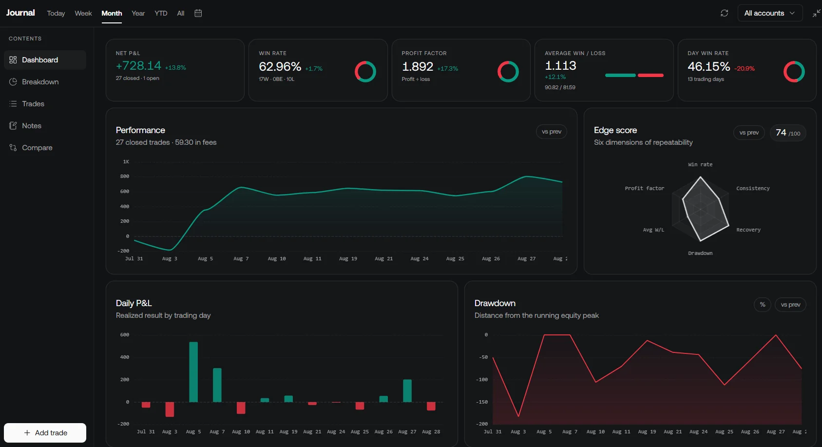
Review compatible recorded trades in LuxAlgo's native journal, keeping backtest, paper and actual results distinguishable. Journal summaries help investigate outcomes but are not a substitute for a broker's current positions or a complete execution log. Organize baseline charts and experiments in a workspace so comparisons remain traceable.
Video: Measuring Strategy Performance in MT5
The retained Darwinex tutorial, published November 5, 2020, discusses equity-curve smoothness, Pearson correlation and R-squared in an MT5/MQL workflow. It provides additional context on performance measurement rather than a formula guide to all seven metrics above. A smooth fitted equity line is not evidence that a strategy will avoid future losses.
A Repeatable Review Checklist
Before comparing reports, align dates, return frequency, cash flows, exposure, costs and equity sampling. Confirm the formulas, denominators and treatment of open or breakeven trades. Review the underlying trades and equity curve, then evaluate later data and realistic execution scenarios. Use the metrics to ask better questions about the strategy, rather than searching for one number that authorizes live trading.
Frequently Asked Questions
Which backtesting metric is most important?
No single metric is sufficient. Review return, drawdown, trade outcomes and risk-adjusted measures together, after checking data, costs, execution assumptions and the evaluation period.
Is maximum drawdown the most I can lose?
No. It describes the largest observed peak-to-trough decline in the selected equity history. Future losses can be larger, and the result depends on whether the data include open positions and intraday valuations.
Does a high win rate mean a profitable strategy?
No. Average win and loss sizes, trade costs and the distribution of outcomes matter. A lower-win-rate strategy can have positive expectancy, while a higher-win-rate strategy can lose money.
Why can two platforms report different Sharpe or Sortino ratios?
They may use different return frequencies, benchmarks or targets, annualization methods and denominator conventions. Align the underlying calculations before comparing the values.
How can I use LuxAlgo to review backtest results?
Use native charts and Quant to inspect a defined strategy, review the code and run it manually. Keep its settings with the results and distinguish native research, legacy tools and actual recorded trades.
Read next