Understanding Moving Averages and How Traders Use Them
Moving averages summarize a price series by combining observations with defined weights. Traders use them to describe trends, compare price with a smoothed reference and build explicit strategy rules. Smoothing changes responsiveness; it does not reveal future prices or guarantee a profitable signal.
The simple moving average (SMA), exponential moving average (EMA) and linearly weighted moving average (WMA) differ in how they distribute those weights. Understanding their formulas helps explain both familiar chart behavior and less obvious relationships with momentum and linear regression.
Define the Input Before Comparing Averages
Let P(t) be the selected price at bar t and n a positive integer period. The formulas below assume consistently spaced bar observations and complete inputs. A period counts observations, so 20 five-minute bars and 20 daily bars summarize different horizons. Session gaps also affect elapsed calendar time.
Record the price source, period, chart interval, initialization and handling of missing values. Some tools expose additional settings such as offsets or smoothing methods. Two lines with the same period number need not use the same calculation or become available at the same time.
| Average | Calculation | Weighting |
|---|---|---|
| SMA | SMAₙ(t) = [P(t) + … + P(t−n+1)] / n | Equal weights across the latest n observations |
| EMA | EMA(t) = αP(t) + (1−α)EMA(t−1) | Recursively decaying weights; a common choice is α = 2/(n+1) |
| Linear WMA | WMAₙ(t) = Σᵢ₌₀ⁿ⁻¹ (n−i)P(t−i) / [n(n+1)/2] | Largest weight on the newest observation, decreasing to the oldest |
For a three-observation example ordered oldest to newest as 10, 12 and 14, the SMA is 12 and the linear WMA is (10 + 2×12 + 3×14)/6, or about 12.67. An EMA also needs its previous state or a specified seed; the latest three prices alone do not uniquely determine a recursive EMA.
SMA Changes Have an Exact Momentum Relationship
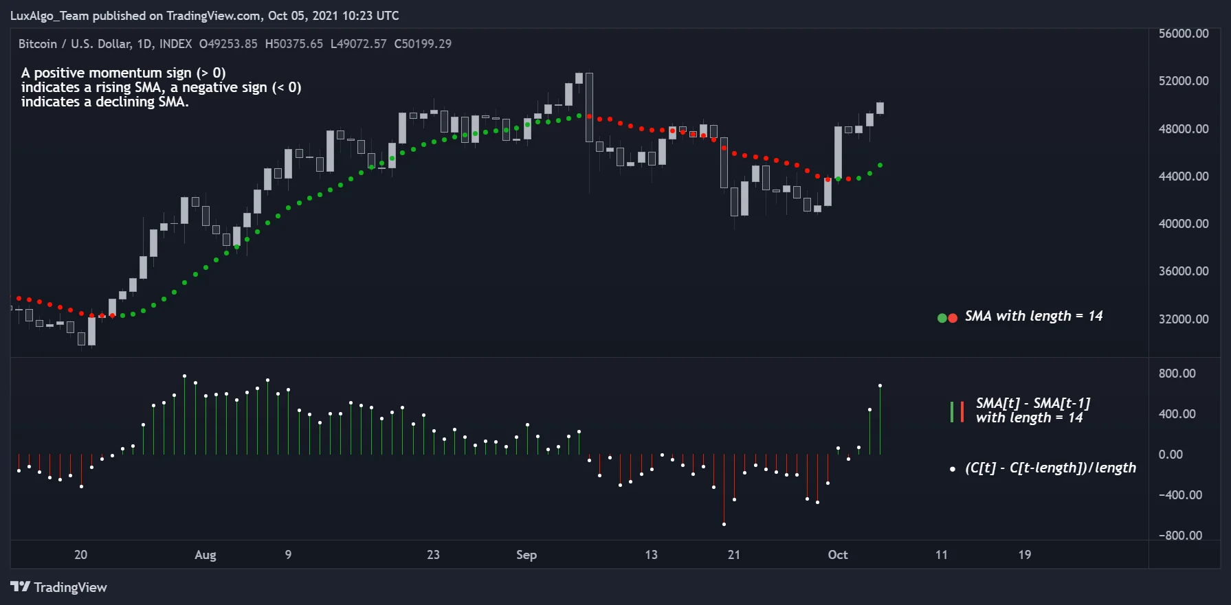
When an SMA advances one bar, one observation enters and one leaves. The shared observations cancel, giving SMAₙ(t) − SMAₙ(t−1) = [P(t) − P(t−n)] / n. This identity uses the same price input and period on both sides.
If the current price exceeds the price n bars earlier, the SMA rises. If it is lower, the SMA falls; if they are equal, the SMA is unchanged. Here, momentum means the absolute price difference P(t) − P(t−n), not RSI or percentage rate of change.
A rolling sum can update the SMA in constant work per new observation after initialization by adding the incoming value and removing the outgoing one. The implementation still needs the outgoing observation and appropriate history or state; constant update work does not mean no storage or initialization cost.
What Lag Means—and What an Offset Does
One useful summary is the weighted average age of the observations. For the SMA, that age is (n−1)/2 bars. For the standard EMA with α = 2/(n+1), its steady-state infinite weighting has average age (1−α)/α, also (n−1)/2. For a linear WMA, the average age is (n−1)/3.
| Method with n = 15 | Average weight age | Important limitation |
|---|---|---|
| SMA | 7 bars | Does not promise every turning point appears exactly seven bars late |
| EMA with α = 2/16 | 7 bars in the steady-state weighting | Different current weight and tail from the SMA despite equal average age |
| Linear WMA | About 4.67 bars | Lower average age does not establish better strategy performance |
Average age is not a universal delay for every frequency, price jump or crossover. The EMA gives more weight to the newest observation than an equal-period SMA, while retaining a decaying tail of earlier information. Different response shapes can coexist with the same average age.
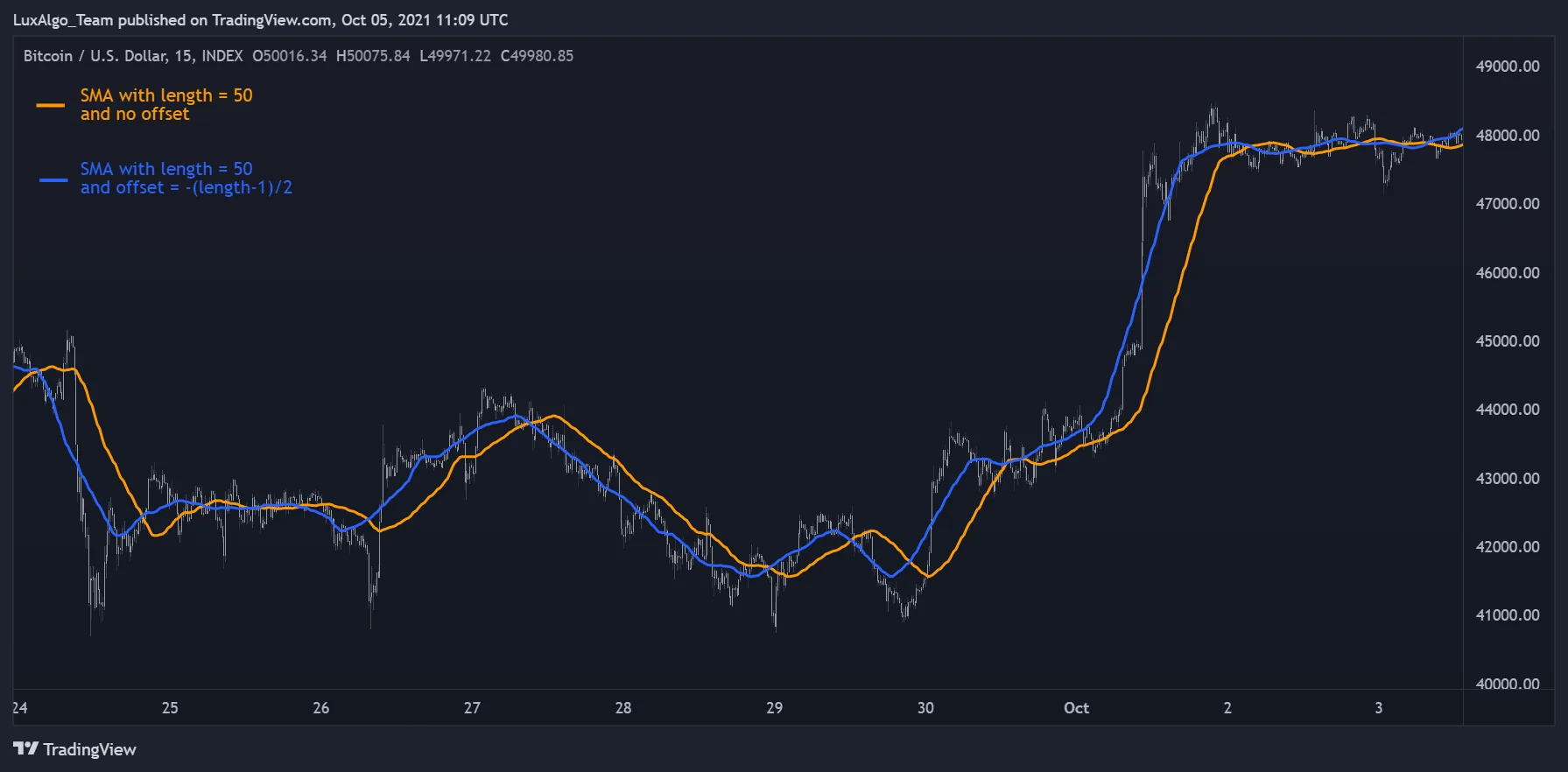
A centered display can make a smoothed line look closely aligned with past price. Treating it as an earlier actionable signal introduces future information. For even periods, the midpoint falls between bars, so the plotting convention also matters. TradingView’s repainting documentation explains related timing issues when later-confirmed values are plotted into the past.
Cascading SMAs Changes Both Smoothing and Delay
Cascading means using one average’s output as another average’s input. Two equal-length SMA stages convolve two uniform weighting sequences, producing triangular discrete weights. Further stages produce increasingly rounded weighting shapes.
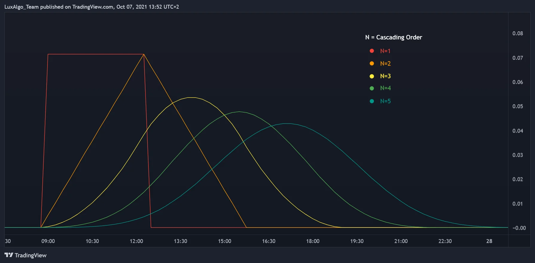
For k stages of length n, the combined finite weighting spans k(n−1)+1 observations and its average age is k(n−1)/2 bars. Three stages of length 5 therefore span 13 observations and have an average age of 6 bars. More smoothing comes with a different response and increased delay.
Repeated discrete uniform convolutions can approach a Gaussian shape after suitable centering and scaling as the number of stages grows. A finite discrete cascade is not literally the continuous Irwin–Hall probability density, although that distribution provides a related continuous-uniform analogy. The distinction matters when implementing exact weights.
EMA Initialization and Zero Denominators
An EMA uses its previous output, so specify how it begins: for example, a first observation or an initial SMA. Different seeds can produce different early values. Their influence decays when 0 < α < 1, but the early portion of a short test can still be affected.
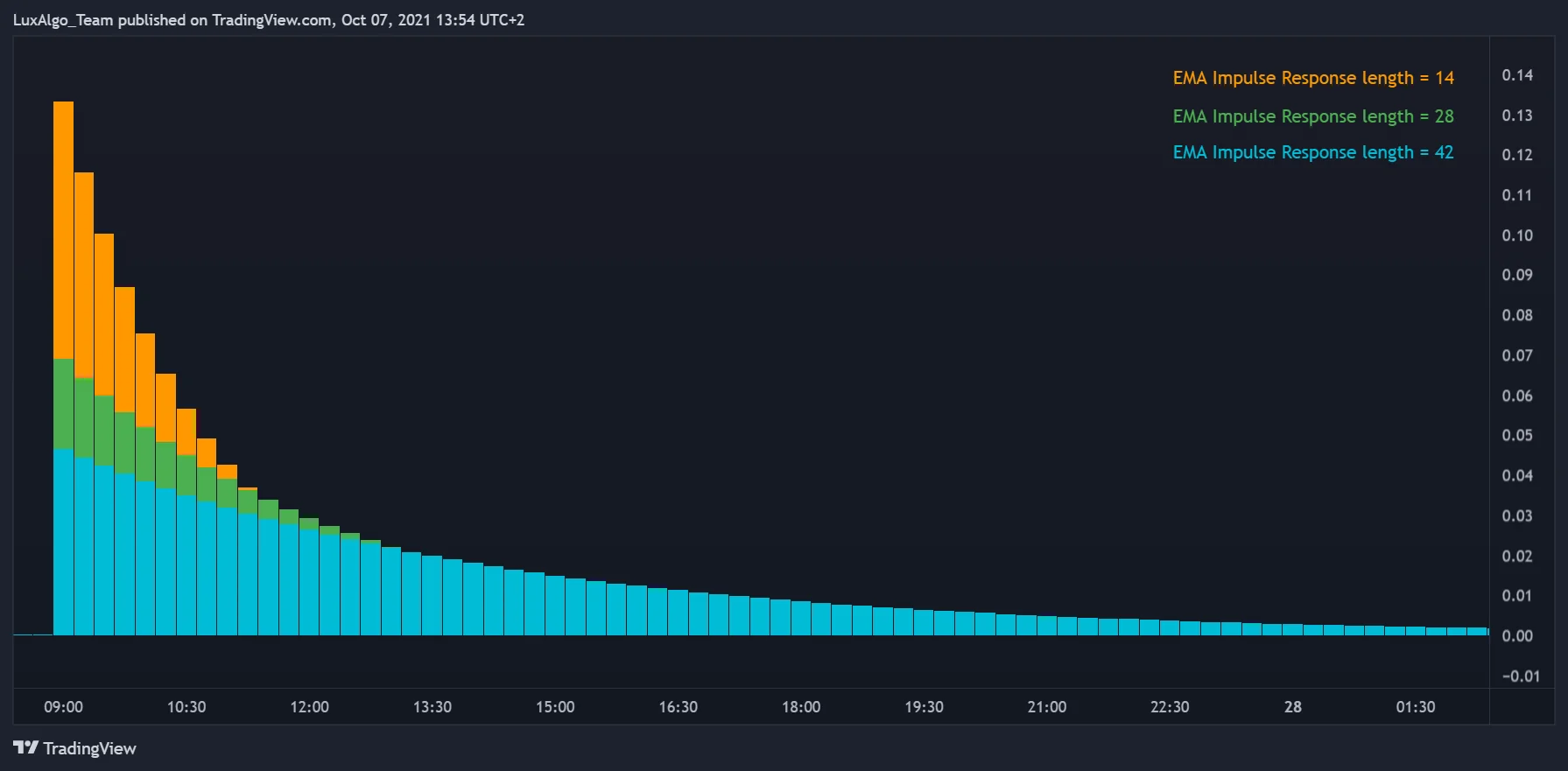
With a strictly positive previous state, nonnegative new inputs and 0 < α < 1, exact arithmetic keeps the next EMA positive. That limited statement does not make EMA smoothing a general safeguard against division by zero. A zero seed followed by zero inputs stays zero; signed inputs can cancel; finite-precision arithmetic can underflow or round very small values.
When an indicator divides by a smoothed quantity, handle zero and near-zero denominators explicitly according to the intended formula. Do not silently turn an undefined ratio into an apparently meaningful trading signal. Also distinguish the common EMA factor 2/(n+1) from other recursive smoothing conventions such as 1/n.
The WMA Has an Exact Relationship with the SMA
For the linear WMA defined above, WMAₙ(t) − WMAₙ(t−1) = 2[P(t) − SMAₙ(t−1)]/(n+1). The SMA on the right is from the previous bar. Replacing it with the current SMA changes the equation.
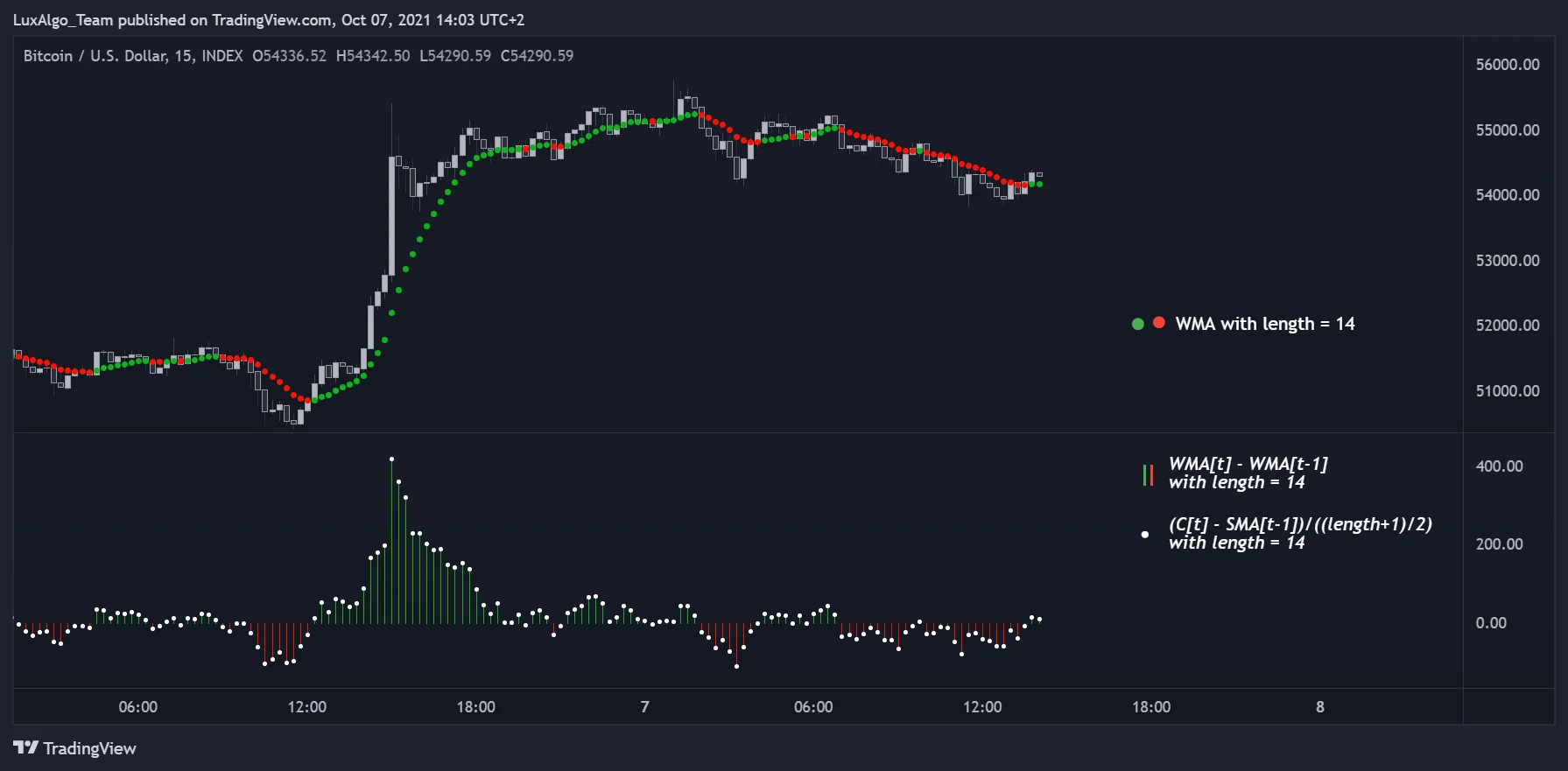
A related result connects the sign of the change in WMAₙ₋₁ with whether current price is above or below SMAₙ. For n ≥ 2, ΔWMAₙ₋₁(t) = 2[P(t) − SMAₙ(t)]/(n−1). The periods differ by one; equality gives a zero change. This is another identity, not an additional independent source of information.
These relationships can support efficient rolling updates once the necessary sums and outgoing values are available. Check initialization, missing observations and numerical behavior when implementing them. A linearly weighted average is one specific weighting scheme; the name “weighted average” alone does not establish these formulas.
Recover a Linear Regression Line from SMA and WMA
For n ≥ 2 equally spaced observations, an ordinary least-squares straight line with an intercept can be expressed using the SMA and linear WMA of that same window. Let S = SMAₙ(t) and W = WMAₙ(t), with the largest WMA weight on the newest observation.
- Fitted value at the oldest observation: A = 4S − 3W.
- Fitted value at the newest observation: B = 3W − 2S.
- Slope per bar: (B − A)/(n−1) = 6(W−S)/(n−1).
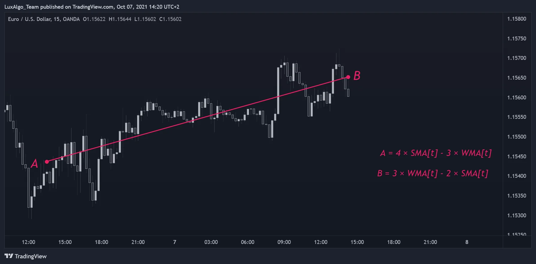
These equations do not automatically apply to irregularly spaced timestamps, different window lengths, a different weighting scheme or regression without an intercept. The oldest fitted endpoint is calculated using the whole current window; drawing it on the oldest bar does not make it an observation that was known then.
Turn the Average into a Testable Trading Rule
A moving average describes data. A strategy also needs entry timing, exits, position sizing and execution assumptions. For a crossover rule, specify whether both values must be confirmed at the close, what price is assumed for execution and how repeated crossings are handled.
A more responsive line may react sooner to some changes while producing more reversals in a choppy sample. A smoother line can suppress some fluctuations while reacting later. Neither property establishes a universally superior average or period. Compare complete rules on the same data, costs and evaluation periods.
- Choose the input, interval, average type, period and initialization before comparing results.
- Record all alternatives tested, including unsuccessful settings.
- Use realistic spread, fees and slippage rather than assuming every signal fills at the plotted value.
- Inspect individual trades and drawdowns, not only aggregate profit.
- Evaluate the selected rule on a later period that was not used to choose it.
- Treat any revision made after viewing that later period as additional development.
Compare Moving-Average Rules in LuxAlgo
Start in Vela, our charting platform, with a specific question about a supported moving-average rule. Keep the symbol, interval, settings and evaluation dates in the research record so the experiment can be repeated.
Ask Quant, our coding agent to help express a supported strategy hypothesis. Inspect the generated code and run it manually. Review strategy settings, costs and individual trades to check that the calculation and information timing match the intended rule.
Check native data coverage and available history. An average needs enough observations to initialize, and changing the symbol or interval changes the experiment and requires another run. The documented US-equity source is Cboe EDGX rather than a consolidated all-venue feed.
Frequently Asked Questions
What is the difference between SMA, EMA and WMA?
An SMA gives equal weight to a finite window. An EMA uses a recursive decay and a specified initial state. A linear WMA gives progressively larger weights to more recent observations in a finite window.
Is an EMA always better than an SMA?
No. Their weighting and response differ, but performance depends on the complete strategy, market, costs and evaluation method. A stronger historical result does not establish universal superiority.
Does shifting an average backward remove trading lag?
No. It changes where later-calculated values appear on the chart. Those values were not necessarily available at the earlier displayed time.
Can an EMA denominator still be zero?
Yes. Zero initialization with zero inputs, signed-value cancellation and finite-precision behavior can produce zero or near-zero values. Handle these cases explicitly in the calculation.
How can LuxAlgo help compare moving averages?
Use Vela and Quant to express a supported strategy rule. Inspect generated code and run it manually, then review costs, individual trades and a later evaluation period.
Read next