Seq2Seq Models for Time-Series in Trading

A sequence-to-sequence (Seq2Seq) model maps a historical input window to a sequence of future estimates. In trading research, that might mean using the last 60 completed bars to forecast the next five closing prices, returns, or volatility readings. The architecture can represent complex relationships, but a lower forecasting error does not by itself establish a profitable trading strategy.
A useful workflow separates model development from trading-rule evaluation. Train and validate the neural network in an appropriate machine-learning environment. Use LuxAlgo’s native charts and Quant, our coding agent, to investigate transparent indicator or strategy baselines and review their behavior on the chart. Quant’s documented Pine Script® workflow should not be confused with training an arbitrary external Seq2Seq network.
How Encoder–Decoder Models Work
The encoder reads the input sequence and produces a learned representation. The decoder uses that representation to generate an output sequence, whose length can differ from the input. The foundational sequence-to-sequence learning paper used one LSTM to encode a sequence and another to decode it, originally for machine translation.
For a market example, define each input row as the features available after a completed daily candle: returns, a volume measure, and selected technical indicators. With 60 rows and 10 features, one sample has a 60 × 10 input shape. A five-step, single-target forecast has five output values. Those dimensions describe the experiment; they are not recommended settings for every market.
Information available at time t
Completed bars t−59 through t → encoder representation → decoder
Forecasts produced at time t
Estimated targets for t+1, t+2, t+3, t+4, and t+5
Define the target before training. Predicting the next five prices is different from predicting five one-bar returns or five cumulative returns measured from the current close. The conversion from forecasts to orders must use the same definition.
Attention and the Context Bottleneck
A basic encoder–decoder compresses the input into a fixed representation. Attention lets a decoder consult different encoder states when producing each output. Bahdanau, Cho, and Bengio’s attention research addressed this bottleneck in translation.
In financial forecasting, attention is a modeling choice to test. It does not automatically remove noise, reveal a causal market driver, or improve every forecast horizon. A prominent attention weight also does not prove that changing the corresponding feature would cause a price move.
Video: Seq2Seq Architecture Explained
StatQuest with Josh Starmer explains the encoder–decoder idea using sequence translation. This is an architecture tutorial, not evidence of a profitable financial forecasting model.
LSTM, GRU, Transformers, and Hybrid Models
LSTM and GRU cells use gates to manage information through recurrent computations. Their design helps address the difficulty of learning long dependencies, but neither guarantees that a weak market signal can be learned reliably.
| Architecture | Main distinction | What to compare in your experiment |
|---|---|---|
| LSTM encoder–decoder | Separate cell and hidden states; input, forget, and output gates | Forecast error, training stability, parameter count, and inference latency |
| GRU encoder–decoder | Reset and update gates; no separate LSTM-style cell state | Whether its smaller matched-width parameterization helps within your compute budget |
| Attention-based model | Uses learned weights to access relevant representations | Improvement over the same baseline without attention |
| Transformer forecaster | Uses attention rather than requiring recurrent processing of every input step | Context length, memory use, forecast horizon, and actual runtime |
| Hybrid model | Combines components such as statistical smoothing and neural networks | Whether each added component helps on untouched future data |
The PyTorch LSTM and GRU documentation specify these recurrent structures. GRUs commonly use fewer parameters than ordinary LSTMs with matched input and hidden widths, but training speed and accuracy also depend on implementation, hardware, sequence length, and tuning. A five-second difference in one run would not establish a general winner.
What Recent Forecasting Architectures Actually Change
Transformer research includes several distinct approaches. These are related time-series forecasting architectures, not all interchangeable versions of a classic recurrent Seq2Seq model:
- PatchTST divides a time series into patches and uses a channel-independent design with shared weights.
- iTransformer embeds individual variables’ histories as tokens and applies attention to relationships between variables.
- Crossformer models dependencies across both time and dimensions through segment embeddings and a hierarchical encoder–decoder.
The original methods do not all process financial news or textual data. A multimodal extension requires a separate text representation, a fusion design, and publication timestamps that reflect when the information was available. Benchmark forecasting results are not automatically stock, forex, or crypto trading results.
Transformers can parallelize substantial training computation, but it is too broad to call every Transformer faster than every recurrent model. An autoregressive decoder may still generate outputs sequentially, and longer contexts can increase memory and compute requirements.
Hybrid models are also worth evaluating. Smyl’s ES-RNN combined exponential smoothing with recurrent networks and won the M4 forecasting competition. That supports investigating hybrid designs; it does not establish a tradable edge on a particular security.
Prepare Data Without Leaking the Future
Choose the symbol, venue, bar interval, session, input features, and target horizon before comparing architectures. Align every feature to its real availability time. A revised economic release or a news item published after the decision cannot be treated as if it were already known.
- Split chronologically. Reserve later periods for validation and a final untouched test. Use validation for model selection and early stopping.
- Fit preprocessing on training data. Estimate scalers and learned imputers within each training fold, then apply those fitted transformations to later data.
- Check every target window. A training sample is not eligible if any of its future labels crosses into the held-out period.
- Keep features causal. Rolling indicators may use completed history; centered smoothing or future-confirmed pivots must not silently introduce later observations.
- Repeat in time order. In walk-forward evaluation, retrain only on information available at each scheduled retraining date.
For example, suppose training data ends at observation 1,000 and the model predicts five steps ahead. The latest training forecast origin is 995, because its labels are 996–1,000. At origin 1,000, an input window covering 941–1,000 can produce forecasts for 1,001–1,005. Historical context shared with training is not itself leakage; using those future targets to fit the model would be.
TimeSeriesSplit provides ordered folds and an optional gap. Choose the gap and sample construction around your label horizon and data timing rather than assuming a default split removes every overlap. TensorFlow’s forecasting tutorial demonstrates chronological partitions, training-only normalization, and single-shot versus autoregressive predictions.
Bidirectional Encoding Is Not Permission to Use Future Prices
A bidirectional encoder can traverse a fully observed historical window in both directions: all those observations are available at the forecast origin. It cannot use data beyond that origin when generating a genuine historical forecast.
This matters when reading research. The attention-based Seq2Seq imputation study reconstructs missing values using observations before and after a missing segment. Its imputation comparisons with methods such as ARIMA and KNN are not evidence that the same method predicts unseen market prices. Information available for reconstructing an old gap may be unavailable for making a live decision.
Match Decoder Testing to Real Inference
With teacher forcing, an autoregressive decoder may receive the true previous target during training. At inference, those future targets are unknown, so the model must use its own earlier predictions. Evaluate the complete forecast path that way; otherwise the reported accuracy can be too optimistic.
Scheduled sampling research addresses this training/inference mismatch, but it is not a universal fix. Also distinguish known future covariates, such as a calendar date, from unknown future prices, realized volume, or news.
Measure Forecast Accuracy and Trading Performance Separately
Report forecast errors by horizon as well as in aggregate. A model can perform acceptably one step ahead and deteriorate over the remaining forecast path. Evaluate all models on the same targets, units, timestamps, and eligible observations.
| Metric | Meaning | Limitation |
|---|---|---|
| MAE | Mean absolute difference between forecast and actual value | Depends on the target’s units and scale |
| RMSE | Square root of the mean squared forecast error | Penalizes large errors more heavily; does not measure profitability |
| MAPE | Mean absolute error divided by the actual value, expressed as a percentage | Undefined at zero and unstable near zero; poorly suited to returns near zero |
| Trading results | Net returns, drawdown, turnover, exposure, and trade distribution | Depend on the rule converting forecasts into orders and on execution assumptions |
See Forecasting: Principles and Practice for point-forecast error definitions and percentage-error limitations. RMSE is not simply the standard deviation of errors, and a low error on normalized values cannot be interpreted as a dollar profit.
Illustrative calculation: actual future prices are 101, 102, and 100; forecasts are 100, 103, and 102. Absolute errors are 1, 1, and 2, so MAE is 4/3 ≈ 1.33 price units. Squared errors are 1, 1, and 4, so RMSE is √2 ≈ 1.41. Neither calculation specifies when to enter, how much to trade, or what it costs.
Compare against simple forecasting baselines, including the latest observed price for a price-level target or zero for a return target. Add a suitable statistical or linear model before assuming a neural architecture earns its extra complexity. For probabilistic forecasts, assess interval coverage and width or an appropriate distributional score; a narrow forecast band is useful only if its uncertainty is credible.
A Forecast Needs an Executable Trading Rule
Specify when predictions become available, the entry threshold, order type, position size, exit rule, and treatment of overlapping forecasts. If a signal is calculated after a candle closes, a simulation must not silently assume an earlier fill at a price that was no longer available.
Suppose a model forecasts a 0.20% gross move and estimated round-trip costs are 0.15%. The difference is only 0.05 percentage points, or five basis points, before forecast error and unexpected execution costs. That arithmetic is a screening consideration, not a prediction that the trade will earn five basis points.
An older Alex Honchar backtesting tutorial reported an illustrative Litecoin portfolio moving from $10,000 to $10,053, a 0.53% increase. Treat it as a tutorial example, not independently verified live performance or validation of Seq2Seq generally. Any comparison requires checking its exact return calculation, cost assumptions, and evaluation period.
Use Quant to Establish a Transparent Chart-Based Baseline
Before adding a neural forecast, establish what a simple rule does on the market you intend to study. In LuxAlgo’s native workspace, ask Quant for a clearly specified strategy, review its code, and run it on the active chart. The strategy creation workflow supports explicit entries, exits, and risk rules.
Build a long-only baseline using completed candles: enter after the 20-period EMA crosses above the 50-period EMA and exit after the opposite crossover. Allow one position at a time. Expose both lengths as inputs and make the simulated order timing explicit.
Then configure commission, slippage, order size, and starting equity. Inspect the backtest viewer and trade log, rather than relying on a headline win rate. Save the run with its symbol, timeframe, inputs, and simulation settings.
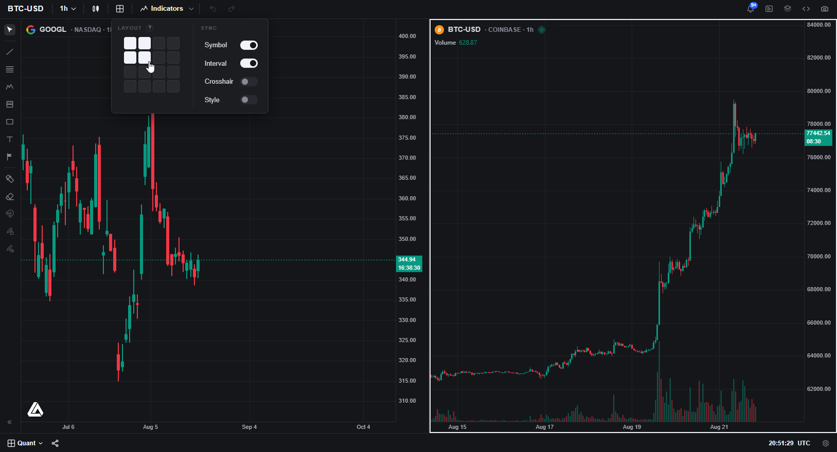
A baseline is useful only if the later comparison matches its opportunity set, data, costs, and execution timing. If the external model uses a different feed or session, reconcile that difference before comparing results.
Training and serving a PyTorch or TensorFlow network remains an external modeling workflow. Do not assume that a trained model, its weights, or its prediction stream can be loaded directly into Quant. LuxAlgo’s Strategy Alerts is a separate legacy product for TradingView toolkit strategies; its webhooks do not establish a general deployment route for an arbitrary Seq2Seq model.
Build, Monitor, and Re-Evaluate the Model
PyTorch or TensorFlow can supply neural-network components; pandas and NumPy help prepare arrays; Matplotlib or Plotly can visualize forecast errors. Indicator libraries can help calculate features, but confirm each feature’s formula, warm-up period, and timestamp. These components do not collectively guarantee a production trading system.
Preserve the fitted preprocessing, model weights, software versions, feature definitions, and evaluation dates. Monitor stale or missing data, prediction latency, forecast error, exposure, and execution failures. Define what happens when required inputs are absent instead of silently generating an order from incomplete data.
Retraining should follow a specified schedule and evaluation process. Updating weights with newer data does not ensure improvement under a market regime change. Retain an earlier version for comparison, test revised models on later observations, and keep the final holdout separate from repeated tuning.
The strongest evidence for a Seq2Seq trading application is a reproducible evaluation that survives realistic costs and later data. Architecture names, favorable charts, electricity-load benchmarks, and impressive in-sample fits are useful research context, but none substitutes for that test.
Read next