Win Rate and Risk/Reward: Connection Explained

Win rate and risk/reward must be read together. Winning frequently can still lose money if losses are large, while a strategy that loses more often than it wins can have positive expectancy when its average winners are sufficiently larger. Costs, position size and the reliability of the sample also matter.
The crucial distinction is between a planned risk-to-reward ratio and realized average wins and losses. A 1:3 target drawn on a chart does not mean the strategy actually earns three units on its winning trades. Use LuxAlgo’s AI trading and charting platform to define and test rules with native charts and Quant, then review actual trading records in the Journal.
Explaining Win Rate and Risk/Reward
What Is Win Rate?
Win rate = winning trades ÷ total trades × 100. If 40 of 100 closed trades are profitable, the win rate is 40%. Define what counts as a trade and whether profit is measured before or after costs before comparing reports.
Partial exits can be grouped as one completed position or counted as separate transactions, depending on the system. Break-even trades also affect the denominator. Keep those conventions consistent; otherwise, two platforms may report different win rates for the same activity. See the LuxAlgo Library’s win-rate reference for the core definition.
What Is Risk/Reward?
This guide uses risk-to-reward: risking $100 to target $300 is 1:3. The equivalent reward-to-risk ratio is 3:1. State the convention because resources sometimes use “risk/reward” for either ordering.
For a long trade, compare entry minus stop with target minus entry. For a short trade, compare stop minus entry with entry minus target. A 10-point planned loss and 20-point target gain give a 1:2 ratio before costs and execution differences.
When reviewing results, use a different measure: average realized win ÷ average realized loss, with losses expressed as positive magnitudes. A strategy can target 3R but realize average wins of only 1.5R after early or partial exits. R should be defined consistently as a unit of risk.
A Ratio Does Not Classify the Whole Trade
A 1:2 target is not automatically conservative, and 1:3 is not automatically aggressive. Exposure, leverage, liquidity, exit distance and the probability of reaching the target all influence risk. Moving a target farther away changes the strategy; it does not improve the outcome by arithmetic alone.
Calculate Expectancy from Realized Outcomes
CME Group’s expectancy lesson explains why the frequency and average size of wins and losses must be evaluated together. For a model using outcomes before costs:
Net expectancy per trade = win rate × average win − loss rate × average loss − average cost per trade.
With a 40% win rate, $300 average win and $100 average loss, expectancy before costs is 0.40 × $300 − 0.60 × $100 = $60 per trade. If average costs are $6, the net estimate is $54. These are hypothetical realized averages, not a projection based only on a planned target.
In this two-outcome example, loss rate equals one minus win rate. If the dataset includes break-even trades, calculate the actual loss fraction rather than assigning every non-winning trade a loss. If wins and losses are already net of all costs, do not subtract those costs again. A direct cross-check is total net profit divided by the same total trade count.
Find the Break-Even Win Rate
For a two-outcome model with average win W, average loss L and average cost C, the break-even win rate is (L + C) ÷ (W + L). The familiar 25% threshold for 3R wins and 1R losses assumes those average outcomes are realized and ignores costs.
| Average win / average loss | Break-even before costs | With 0.10R average cost |
|---|---|---|
| 0.8R / 1R | 55.56% | 61.11% |
| 1R / 1R | 50% | 55% |
| 2R / 1R | 33.33% | 36.67% |
| 3R / 1R | 25% | 27.5% |
Be careful when translating percentages into whole trades. With exactly 100 trades, $200 wins and $100 losses, 33 wins produce −$100 before costs, while 34 wins produce +$200. Neither is exact break-even. With $300 wins and $100 losses, 25 wins and 75 losses produce exactly $0 before costs.
Clearing Up Misconceptions
Why a High Win Rate Is Not Enough
Suppose 70 of 100 trades win $50 and 30 lose $100. The result is $3,500 − $3,000 = $500 before costs, or $5 per trade. At $6 average cost per trade, that becomes a $100 net loss over the sample. The strategy wins often, but its average advantage before costs is small.
Large occasional losses can be especially important. A win-rate statistic counts a small win and a large win equally; it also counts a small loss and a severe loss equally. Review the loss distribution, maximum drawdown and exposure rather than relying on one percentage.
Why a Large Target Is Not Enough
A distant profit target may produce large winners when reached but a lower win rate. If a filter raises win rate while reducing average wins, net expectancy may improve or worsen. Evaluate the complete result instead of maximizing either metric in isolation.
Likewise, winning fewer than half of your trades does not imply inevitable losses. A 40% win rate with realized $300 average wins and $100 average losses has positive expectancy before costs. Whether an actual strategy can sustain those outcomes requires evidence.
Positive Sample Expectancy Is Not a Guarantee
A positive estimate describes the observed sample and its assumptions. It does not establish that future expectancy will be positive or that returns will be steady. Ten trades and a thousand trades can show the same win rate while providing very different amounts of evidence; even a large sample can be misleading if it comes from one unusual market regime or a heavily optimized test.
Compare Trading Outcomes Fairly
The following examples use 100 trades, fixed $100 average losses and the stated average win amounts. They illustrate arithmetic, not verified results for high-frequency trading, trend following or any named strategy. The $6 cost assumption is included only to show its effect.
| Illustrative model | Win rate | Average win / loss | Result before costs | After $6 cost per trade |
|---|---|---|---|---|
| A | 76% | $80 / $100 | +$3,680 | +$3,080 |
| B | 40% | $300 / $100 | +$6,000 | +$5,400 |
| C | 60% | $50 / $100 | −$1,000 | −$1,600 |
Model B has the largest sample profit here, but the table does not establish the best strategy. It omits holding time, capital requirements, drawdown, execution difficulty and the order of returns. Comparing 100 trades across different time periods is also different from comparing returns over the same calendar period.
If position sizes vary, dollar expectancy may be dominated by the largest trades. Review dollar outcomes alongside consistently calculated R-multiples and account-level results. A simple fixed-dollar example is not a compounded equity forecast.
Use LuxAlgo to Review Both Metrics
Define a Baseline on Native Charts
Start with the relevant instrument, interval and session on LuxAlgo’s native charts. Describe the setup with a small number of explicit conditions. If adding a trend or volume filter, state why it might change outcomes before looking at the backtest.
Compare One Rule Change with Quant
Quant is LuxAlgo’s coding agent for creating and refining indicators and strategies. Ask it to implement explicit entry, exit and sizing rules, then review Code and inspect the simulated trades after running the script.
- Preserve the baseline: record the original rules, sample, instrument and interval.
- Change one condition: compare a specific filter or exit variant while retaining the other assumptions.
- Inspect implementation: check signal timing and whether only information available at the decision time is used.
- Compare the full report: examine net result, trade count, win rate, average outcomes and drawdown together.
- Validate separately: evaluate the selected change on data not used to choose it, then monitor forward results.
Use Quant’s strategy controls to check capital, order size, commissions and slippage. A script compiling successfully does not verify its trading logic, and a strong historical result does not guarantee a live edge.
Native chart alerts need separate configuration. Saving a Quant strategy does not automatically run it across every watchlist symbol or place broker orders. Keep research, notifications and execution distinct when interpreting a strategy’s results.
Use the Journal for Actual Fills and Decisions
Backtests describe simulated execution under assumptions. The native Journal helps review recorded trading activity. Compare actual entries, exits, size and costs with the plan to identify whether differences come from the rule, execution or discretionary changes.
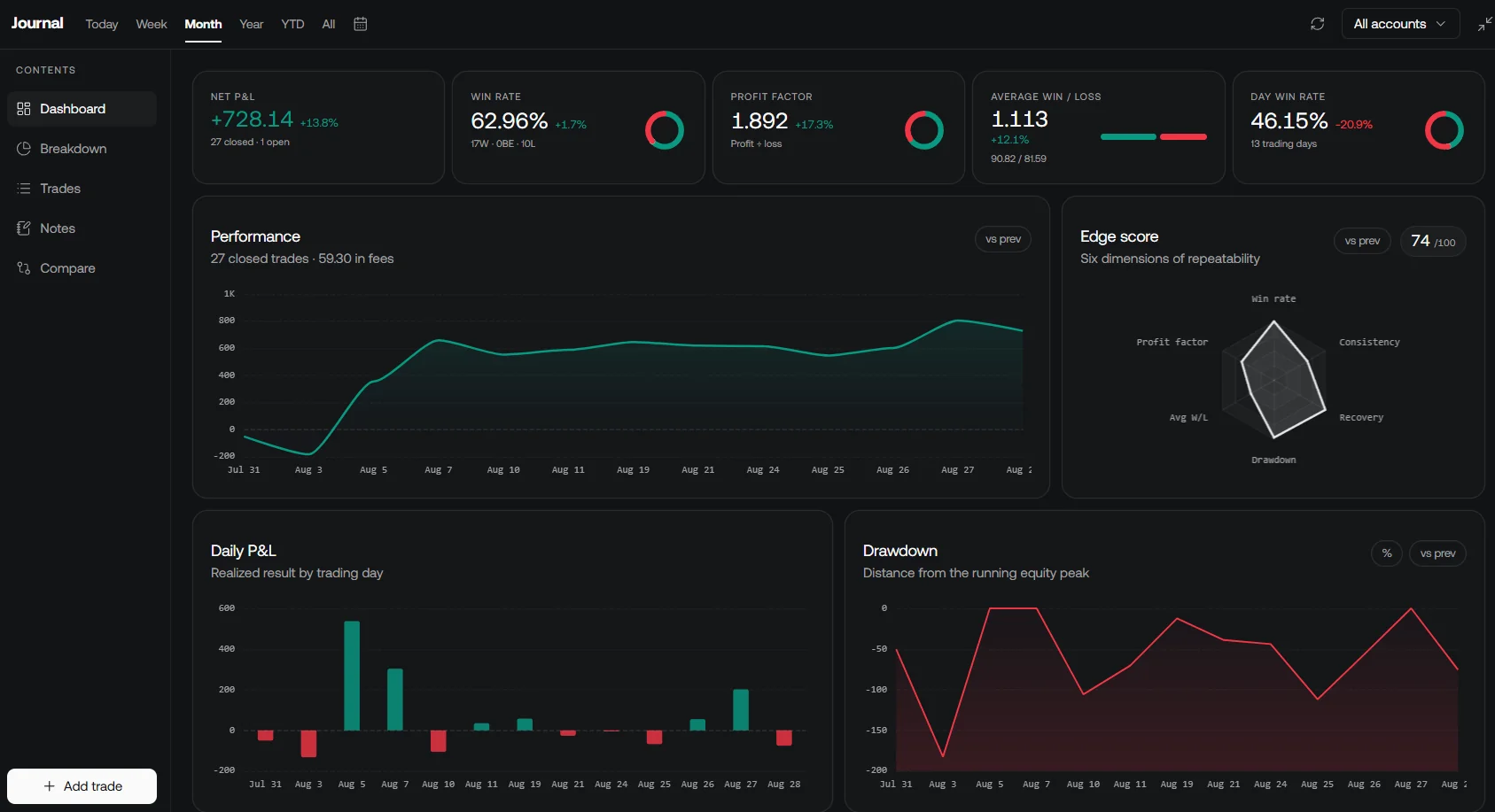
Journal accounts support manual records, supported file imports and broker connections where available for the account. Check completeness, timezones, duplicate trades and costs before comparing analytics.
| Observed change | Possible explanation to investigate |
|---|---|
| Win rate rises but net result falls | Smaller average winners, larger losses, higher costs or changed exposure. |
| Win rate falls but net result rises | Larger winners or smaller losses may offset the lower hit rate. |
| Backtest and actual results diverge | Different fills, costs, timing, sizing, data or rule compliance. |
| A filter looks excellent on a few trades | Insufficient evidence, concentration in one regime or selection after many trials. |
Keep TradingView Comparisons Consistent
Pine Script® runs on LuxAlgo through PineTS. If the same script also runs on TradingView, compare settings, data, sessions and simulated fills; different runtimes do not produce identical statistics.
Community feedback can help identify unclear rules or overlooked assumptions. Ask for critique of the test design and losing examples as well as winning screenshots. Agreement from other traders cannot substitute for evidence from a consistent sample.
Review the Process as Markets Change
Review at a cadence that fits the strategy’s trading frequency. Compare periods with consistent definitions and note changes in market conditions, execution and costs. Avoid repeatedly changing targets after individual losses or selecting a new parameter solely because it has the best recent win rate.
Keep risk limits separate from the desire to improve statistics. Widening a stop can change both loss size and win rate; recalculate exposure rather than treating the higher hit rate as reduced risk. As the SEC’s stop-order bulletin explains, actual fills can occur away from a stop trigger, and stop-limit orders can remain unfilled.
The aim is a strategy whose net outcomes are supported by evidence and compatible with the risk taken. Win rate and average win/loss size help explain those outcomes, while costs, drawdown and sample quality determine how much confidence to place in them.
FAQs
Is a 60% win rate good in trading?
It depends on average wins, average losses, costs and risk. At 60% wins, $50 average wins and $100 average losses produce −$10 per trade before costs. A lower win rate can produce a better result if average winners are sufficiently larger. The percentage alone cannot establish strategy quality.
What is the difference between risk/reward and win rate?
A planned risk-to-reward ratio compares the intended loss with the target gain on a trade; win rate measures the share of trades that win. To evaluate expectancy, combine win rate with realized average wins and losses, using a consistent treatment of costs. A planned 1:3 ratio does not guarantee the strategy will realize 3R average winners.
Read next