Reinforcement Learning for Portfolio Rebalancing

Reinforcement learning can learn a policy for changing portfolio weights, but it must earn its place against simpler rebalancing rules after costs. An agent selects allocations from the information available at a decision time and receives feedback from a simulated environment. Its results depend on the data, reward, constraints and execution assumptions you give it.
That is different from an agent automatically learning profitable decisions from live markets. Most research begins with historical training and separate evaluation. A fixed trained policy can produce different allocations as its inputs change without updating its parameters. Online learning is an additional design choice that needs its own controls.
- Define the task: choose the assets, decision schedule, permitted weights and execution timing.
- Build the environment: account for holdings, cash, costs and information availability.
- Compare fairly: evaluate against buy-and-hold, scheduled and threshold-based rebalancing under the same assumptions.
- Keep the tools distinct: use a dedicated RL environment for portfolio training and LuxAlgo charts and Quant for relevant chart-based research and rule testing.
How the Agent–Environment Framework Works
A rebalancing policy maps an observation to an action. The observation might include current holdings, cash, recent returns, volatility estimates and correlations. The action can be a target allocation, an order adjustment or a decision to leave the portfolio alone. The environment translates that action into trades, updates portfolio value and supplies a reward.
The sequence matters: observe available information → choose an action → simulate executable trades and costs → observe the next outcome. If a feature uses today’s closing price, the test must not assume an earlier fill that was available before that close was known. Define the decision and fill timestamps explicitly.
Calendar rebalancing restores a target mix on a schedule. Threshold rebalancing acts when weights drift beyond a stated band. Mean-variance methods can also be recalculated with changing estimates and constraints. RL adds a learned sequential decision policy; adaptability is not exclusive to RL, and greater complexity does not establish better results.
Design States, Actions and Rewards
Use information that existed at the decision time
Start with a small, interpretable observation set. Include the current portfolio because the cost of moving to a target depends on what is already held. Align market timestamps, corporate actions and cash flows. For earnings and economic releases, use their actual availability dates rather than assuming revised values were known historically.
More features can add noise, missing values and opportunities to overfit. Fit normalization and feature-selection choices on training data. Carry those fitted transformations into validation and testing without using future observations. Current index membership applied to old data can also introduce survivorship bias.
Make the allocation feasible
A simple research task might allow long-only holdings plus cash, with nonnegative weights summing to one. For example, 10% cash and 30% in each of three assets is a feasible allocation under those rules. It is an illustration, not a recommended portfolio.
A vector of independent bounded outputs does not automatically satisfy the total-weight constraint. Define how model outputs become feasible targets and how concentration limits are enforced. Softmax can create positive weights summing to one, but it does not by itself enforce a maximum holding size. Shorting and leverage require different exposure, financing and margin rules.
Translate target weights into orders using actual holdings, current prices, rounding and available cash. Model rejected or partially filled orders and record the allocation actually achieved. A target and an executed portfolio are not necessarily identical.
Reward the intended behavior
A starting reward can be the change in portfolio value after modeled trading costs. A log-return reward, log(Vt+1 / Vt), requires positive values and consistent treatment of external deposits and withdrawals. It measures an outcome over a step; it is not itself a complete risk objective.
Additional penalties might discourage concentration, drawdown or excessive turnover. Put return and penalty terms on documented scales and assess the tradeoff on validation data. A large penalty can make the policy avoid useful trades; a small one can leave the unwanted behavior largely unchanged. A reward penalty is not a hard risk limit.
A Sharpe-based objective needs a defined observation window, excess-return convention and treatment of very low volatility. It is not a meaningful ratio for a single isolated return. Also distinguish the reward optimized during training from the metrics used to judge the final portfolio.
A Worked Rebalancing and Cost Example
Suppose a hypothetical $100,000 portfolio holds $60,000 in asset A and $40,000 in asset B. The chosen target is 50% in each. Ignoring costs for the target calculation, the rebalance sells $10,000 of A and buys $10,000 of B. Total traded notional is $20,000, even though only $10,000 moves from one asset to the other.
At an illustrative all-in cost of 0.10% on each traded dollar, the estimated charge is $20, or 0.02% of portfolio value. A weight-based approximation gives the same result: 0.001 × (|0.50−0.60| + |0.50−0.40|) = 0.0002. Here the absolute-weight sum counts both the sale and purchase; a turnover statistic defined as half that sum uses a different convention.
The simulator must fund the $20 charge and adjust final cash or orders. Exact post-cost weights can therefore differ slightly from the pre-cost target. Include spreads, commissions and slippage consistently, without charging the same component twice. Larger or less liquid trades may require a size-dependent impact model; this flat-rate illustration is not a universal cost estimate.
If the post-trade asset returns were hypothetically +2% and −1%, an exact 50/50 allocation would earn 0.5% before costs for that period. The unrebalanced 60/40 mix would earn 0.8%. This single example demonstrates that restoring a target need not maximize the next period’s return. Evaluate the full risk and return objective over a suitable sample.
Choose an Algorithm That Fits the Action Space
The Stable Baselines3 algorithm table documents action-space support. Choose an implementation compatible with the environment before comparing results. No algorithm name establishes suitability for every portfolio.
| Method | Possible allocation design | Important distinction |
|---|---|---|
| DQN | Choose among a finite menu of target portfolios or actions | The standard SB3 implementation uses discrete actions; many assets and finely spaced weights can create an impractically large menu. |
| Proximal Policy Optimization | Learn discrete choices or continuous outputs mapped to valid weights | Proximal Policy Optimization supports both kinds of action space. It is commonly implemented with an actor and critic; it is not a separate alternative to all actor–critic methods. |
| A2C | Use an actor to propose actions and a critic to estimate value | Also supports discrete and continuous actions in SB3. Training stability must be measured for the chosen environment. |
| SAC or TD3 | Use continuous outputs with explicit allocation constraints | SB3 supports continuous Box actions for these methods. Bounds alone do not ensure a valid portfolio. |
The actor determines actions and the critic estimates value to help training. These are learning components, not separate investment advisers. Keep model size and tuning effort proportional to the data, and compare multiple training seeds. SB3 notes that exact reproducibility is not guaranteed across software releases, platforms or CPU/GPU execution.
Implement and Evaluate the Portfolio Environment
1. Write the investment and execution specification
Document the universe, cash treatment, rebalancing frequency, position limits, borrowing assumptions, transaction costs and fill timing. Decide whether the task maintains a strategic target or actively changes that target. Include a no-trade action or explain how the policy can retain existing holdings.
2. Build simple reference strategies first
Run buy-and-hold, equal-weight scheduled rebalancing and a stated drift-band rule on the same data. Where relevant, add a constrained mean-variance or risk-parity reference. Risk parity allocates around estimated risk contributions, not simply equal capital weights. Give each reference the same universe, costs and execution opportunities as the RL policy.
3. Test the environment before training
Use small hand-calculated cases: unchanged prices with no trades, a single rebalance with costs, a deposit, missing prices and a rejected order. Check that portfolio value reconciles with holdings and cash. Confirm that the agent cannot earn rewards through accounting errors, impossible fills or repeated cash flows.
4. Train on an earlier period and tune on validation data
Separate time periods chronologically. Keep the final test period untouched while selecting features, rewards, network size and other settings. Repeatedly training on the same historical episode does not create independent market history. Record software versions, seeds and the complete configuration for each run.
5. Evaluate across periods, costs and seeds
Freeze the selected policy and compare its net returns, drawdowns, volatility, turnover, concentration and benchmark-relative performance. Show the distribution across seeds rather than only the best run. Stress costs, delayed fills, missing data and different market conditions. Preserve the same evaluation budget and assumptions across competing methods.
A walk-forward design can retrain on information available before each new evaluation window. Keep the schedule fixed in advance. If you inspect results and repeatedly redesign the policy using a supposed holdout period, that period has become part of development and is no longer an untouched test.
6. Separate simulated evidence from operational readiness
Out-of-sample results are evidence to assess, not proof that a system is ready to trade. Paper operation can expose data, accounting and execution failures. Any deployment needs monitoring, limits, a fallback allocation and a way to stop the system. Online policy updates add another change process; they should not silently alter a validated policy.
Current Tools for RL Development
- Gymnasium: a maintained fork of OpenAI Gym with a standard environment interface. New work should check the current interface and migration guidance instead of copying old Gym examples unchanged.
- Stable Baselines3: implemented RL algorithms and supporting utilities. Its evaluation guidance emphasizes separate test environments, repeated runs and careful experimental design.
- FinRL portfolio-allocation tutorial: an educational starting point for a weight-allocation environment. The published example assumes long-only stock weights summing to one and explicitly omits transaction costs. Audit those assumptions and package compatibility before reuse.
Choose a compatible deep-learning stack for the RL implementation; using both PyTorch and TensorFlow is not a requirement. Separate backtesting libraries can help with accounting and analysis, but they do not automatically provide a correct RL integration. Validate observation timing, order conversion and reward calculation wherever systems connect.
Research Applications and Their Limits
RL research explores dynamic allocation, hierarchical policies, ensembles and changing objectives. A hierarchy could separate strategic allocation from trade execution. An ensemble could combine several policies. Each adds decisions about constraints, training and evaluation; neither guarantees better stability or returns.
For liability-oriented investing, the environment would need obligations, withdrawals and a horizon, rather than only a stock-return objective. For personalized allocations, it would need explicit investor constraints. These are possible problem designs, not evidence that pension funds or robo-advisers universally use RL successfully.
The May 2024 portfolio-management paper cited in the original article studies learned allocation, but its proposed setting assumes liquidity, fulfilled orders and no transaction charges. Its historical findings should be read within those assumptions. They do not establish live, after-cost superiority for a different portfolio.
Rare stress events remain scarce, market relationships change, and simulated execution can misrepresent liquidity. Complex policies can also be difficult to explain. Maintain allocation and action logs, inspect concentration and turnover, and investigate large changes. Removing manual discretion does not remove bias from data, objectives or model selection.
Watch: Objective-Driven Portfolio Construction
The Fields Institute recording below features Jithin Pradeep and Tina Ruiwen Wang of The Vanguard Group, with a talk dated February 16, 2023. It offers historical research context for objective-driven portfolio construction. It is not a LuxAlgo tutorial or evidence of the performance of your own implementation.
Where LuxAlgo Fits in the Research Workflow
Start with LuxAlgo’s native charts and data coverage to inspect the instruments and market conditions behind a hypothesis. Use Quant, our coding agent to develop explicit chart-based strategy rules. Inspect the generated code and run it yourself before assessing the result.
For example, you might investigate a precisely defined volatility or trend filter that could later be considered as an input in a separate portfolio study. Check its calculation and signal timing first. Native strategy testing can help evaluate explicit supported chart rules with realistic costs and a separate testing period. It does not establish that a multi-asset RL allocation policy has been trained or validated.
Keep portfolio accounting, cross-asset constraints, the RL training loop and whole-portfolio evaluation in the dedicated research environment. A profitable single-instrument backtest cannot be added to other profitable backtests and treated as a feasible shared-capital portfolio. Correlated exposure, capital competition and synchronized fills need portfolio-level treatment.
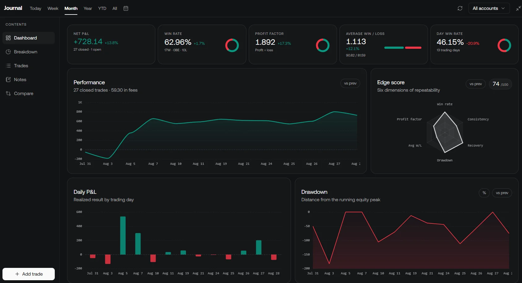
The native LuxAlgo journal helps review supported trade records and trading behavior. Reconcile portfolio holdings, cash flows and allocation performance with the dedicated portfolio ledger rather than assuming a trade journal is a full allocation-risk engine.
Quant codes and backtests explicit chart-based rules; it is not an RL trainer or automatic validation of an arbitrary portfolio agent. Consult the Library, documentation and current plan details for the tools relevant to your specific research step.
Frequently Asked Questions
Does reinforcement learning always outperform traditional rebalancing?
No. It learns a policy under chosen data, rewards and constraints. Compare it with simple rebalancing rules using the same costs, execution assumptions and separate evaluation periods.
Does an RL portfolio agent have to learn continuously in live markets?
No. A trained policy can change allocations when its inputs change while its parameters stay fixed. Online learning is an additional design choice that needs separate validation and controls.
Is Proximal Policy Optimization only for continuous portfolio weights?
No. The Stable Baselines3 implementation supports both discrete and continuous action spaces. Its outputs still need a defined mapping to feasible portfolio allocations.
Why do rebalancing costs need special attention?
A transfer from one holding to another involves a sale and a purchase. Define whether turnover counts one side or both, fund the resulting costs and simulate the actual final holdings.
Can LuxAlgo Quant train and validate a multi-asset RL portfolio agent?
The documented chart workflow supports coding and testing explicit chart-based rules. Keep RL training, shared-capital portfolio accounting and allocation-policy evaluation in a dedicated research environment.
Read next