Time Series Analysis in Algo Trading
Time series analysis studies observations in time order to describe patterns, estimate uncertainty and evaluate forecasts. In algorithmic trading, the target might be a return, volatility, volume or a changing relationship between instruments. Choosing that target comes before choosing a model.
A useful forecast is not automatically a profitable trade. Entry timing, position size, spreads, commissions, slippage and execution constraints determine whether a forecast can support a trading rule. Keep statistical evaluation and trading evaluation separate, then examine how they connect.
- Define the target and horizon: tomorrow’s return and next month’s volatility require different evidence.
- Respect information timing: every feature must have been available when the decision was made.
- Compare simple baselines: complexity must earn its place in an evaluation period.
- Model uncertainty and costs: a small forecast error or high directional hit rate does not establish net profitability.
Understand the Series Before Modeling It
Stationarity is an assumption to assess
A weakly stationary series has a stable mean and variance, with covariance depending on the lag rather than the calendar date. Financial prices and returns can behave differently, and changing volatility or structural breaks can challenge the assumptions. Stationarity does not ensure accurate predictions.
Differencing can remove some forms of nonstationarity; logarithms can change scale and stabilize some variance patterns. Neither transformation is a universal repair. Forecasting: Principles and Practice also warns that excessive differencing can introduce artificial dynamics. Inspect the transformed series and preserve an interpretation of what is being forecast.
The Augmented Dickey–Fuller test has a unit-root null hypothesis. The KPSS test instead starts with stationarity as its null under its specified setup. Lag choices, trend terms, sample size and breaks affect interpretation; failing to reject a null does not prove that the model assumptions will hold in the future.
Autocorrelation and seasonality describe dependence
Autocorrelation measures a series’ relationship with its own lagged values. Partial autocorrelation examines a lag after accounting for intervening lags. These diagnostics can guide model candidates, but a striking plot can also reflect a trend, a short sample or repeated searching.
Seasonality refers to recurring calendar patterns, such as intraday activity around a session boundary. Specify the market calendar and timestamp convention. Do not assume that a pattern found in one period survives changes in liquidity, participants or trading hours.
For example, prices of 100, 102 and 101 imply simple consecutive returns of 2% and approximately −0.98%. A price-level model and a return model therefore answer different questions. Keep transformations, units and forecast horizons consistent when comparing results.
Choose a Method for the Question
| Method | What it represents | Important limitation |
|---|---|---|
| Chart moving average | A trailing weighted summary of observed values | Smoothing introduces lag and does not certify a trend trade |
| AR / statistical MA / ARIMA | Lagged values, lagged innovations and optional differencing | Requires model diagnostics and separate forecast evaluation |
| GARCH family | Conditional variance dynamics | A volatility estimate does not identify price direction |
| RNN / LSTM | Learned sequential relationships | Capacity adds data, tuning and overfitting demands |
| Kalman filter | Recursive state estimation under a state-space model | Results depend on the transition, observation and noise assumptions |
Chart moving averages versus statistical MA models
A simple moving average gives equal weight to observations in a chosen window. An exponential moving average emphasizes recent observations; a weighted moving average follows its specified weights. Faster response can also mean more sensitivity to noise. No average is universally best for volatile or trending markets.
A statistical moving-average model is different: it models the series using current and lagged innovations, or unpredictable errors. An autoregressive model uses lagged values of the series. AR is not synonymous with momentum, and a statistical MA model is not simply a chart-smoothing filter.
The ARIMA model description combines these components. In ARIMA(p,d,q), p is the autoregressive order, d is the differencing order and q is the innovation-lag order. Differencing allows some nonstationary series to be modeled through a stationary transformed process; it does not make every dataset suitable or produce precise forecasts automatically.
Use ACF and PACF as diagnostic inputs, examine residual behavior and evaluate candidate settings without repeatedly reusing the final test period. Compare with a simple forecast such as the latest price for a price-level target. A complicated model can appear accurate merely because prices change little between observations.
GARCH models conditional volatility
A standard GARCH(1,1) model expresses the next conditional variance as a constant plus a contribution from the latest squared innovation and the previous conditional variance. A mean model may be fitted separately. The arch documentation demonstrates this separation and variants that allow asymmetric responses to positive and negative shocks.
EGARCH models log variance, while threshold or asymmetric specifications use different responses to shocks. Their names and parameter conventions depend on the implementation. Compare the intended specification, distributional assumptions and diagnostics rather than assuming a variant handles every crisis better.
Illustrative calculation: use decimal-return units, a constant of 0.000002, shock coefficient 0.10, persistence coefficient 0.85, latest innovation 0.02 and previous variance 0.0001. The next variance is 0.000002 + 0.10 × 0.02² + 0.85 × 0.0001 = 0.000127. Its square root is about 1.127% volatility per modeled period. These hypothetical coefficients illustrate the calculation, not an estimated market forecast or a loss limit.
RNNs and LSTMs learn sequential relationships
Recurrent networks process sequences; LSTM gates are designed to help retain and update information across steps. That capability does not establish superiority over simpler models on financial data. Window length, features, training sample, regularization and model selection all affect results.
The TensorFlow time-series tutorial compares baselines with several neural architectures and computes normalization statistics from training data. Its weather-data results illustrate a workflow, not trading returns. For financial research, fit preprocessing within each training window and evaluate the exact horizon you intend to trade.
Kalman filtering estimates a changing state
A Kalman filter updates a state estimate as new observations arrive, combining a model prediction with observed information. The statsmodels state-space framework supports filtering, smoothing and forecasting. Define the state, observation relationship and noise assumptions before interpreting an estimated trend or relationship.
For a live decision, use information available up to that point. A full-sample smoother can use later observations to revise earlier states; using those revised states as historical trading signals introduces future information. A recursive filter also needs parameters estimated without looking ahead. Fast updating alone does not make a system suitable for high-frequency execution.
Validate Forecasts in Time Order
Use a documented chronological development and evaluation process. An expanding window retains earlier training observations; a rolling window limits training to a recent span. The choice trades off sample size and responsiveness to change. Neither automatically prevents overfitting or dominates a well-designed fixed holdout.
In a walk-forward example, fit through one cutoff, evaluate the following month, then advance the cutoff using only information available at that time. Freeze the tuning and refitting schedule before interpreting the results. The TimeSeriesSplit documentation describes ordered splits, optional training-size limits and a gap before evaluation. Its comparable-duration interpretation assumes equally spaced samples.
A gap must reflect the actual label and information timing. If a training label uses a return that ends inside the evaluation period, chronological row ordering alone has not separated the information. Exclude overlapping training labels where necessary, and account for publication delays in external features.
- Prepare data causally: check missing observations, corporate actions, venue coverage and session boundaries. Interpolation using a later endpoint can leak future information; silently filling a gap can also invent a tradable price.
- Fit transformations within training: scaling, imputation, feature selection and parameter searches belong inside the development process.
- Compare the same target: report units, horizon, sample dates and the baseline alongside the forecast metric.
- Keep a final evaluation: repeated inspection and tuning consume its independence. Track unsuccessful experiments as well as the selected model.
- Check residuals and instability: investigate persistent errors, changing variance and periods when the model fails. More data does not necessarily fix a changing relationship.
MAE summarizes absolute error; RMSE gives larger errors more weight. MAPE is difficult to interpret when the target is zero or near zero, as returns often are. For direction classification, examine class balance and a baseline as well as accuracy or F1. None of these measures includes trading costs by itself.
Trading example: 60 hypothetical winning trades at $10 each and 40 losing trades at $20 each produce a 60% hit rate but a $200 gross loss over 100 trades. Costs make that worse. Forecast evaluation must therefore connect to the payoff, turnover and execution assumptions of the actual rule.
Use LuxAlgo to Review a Testable Chart Hypothesis
Begin with LuxAlgo’s native charts and data coverage to inspect the instrument, timeframe and session context. Keep the data source consistent with the research question. A chart feed and an execution feed may differ.
Ask Quant, our coding agent to implement explicit chart rules. Inspect the generated code and run it yourself. Verify the entry and exit timing, lookback and position logic against the specification before interpreting the equity curve.
Use native strategy testing with standard candles, realistic costs and separate evaluation periods. External ARIMA, GARCH or neural-model research may require its own statistical environment and integration. Do not assume that a chart script reproduces an external fitted model or that a named method is available without checking the actual implementation.
Review compatible trade records in the native LuxAlgo journal alongside model versions and test notes. Reconcile actual execution with broker records. A good forecast and a correctly implemented trade are separate observations.
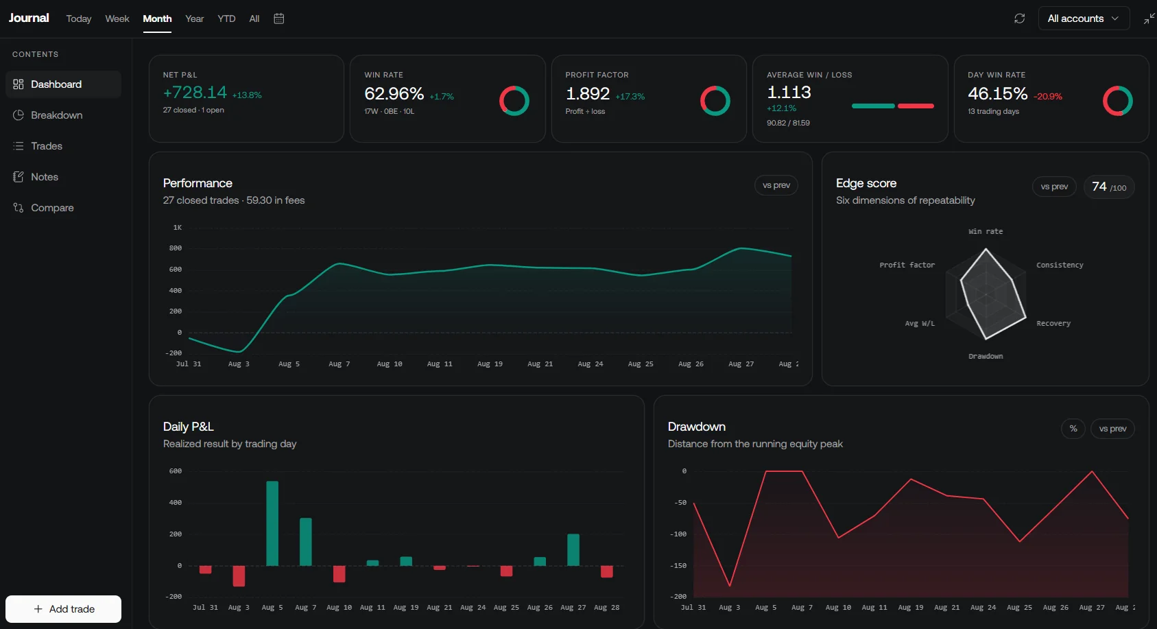
Keep custom Quant development, configuration searches, alerts and live broker execution separate. Use the Library for study ideas.
Translate the Analysis into a Trading Rule
| Research idea | Rule details to specify | What can undermine it |
|---|---|---|
| Moving-average crossover | Completed-bar calculation, entry timing, exit, size and cost assumptions | Lag, whipsaws and selecting favorable lookbacks after many trials |
| Volatility-based exposure | Forecast horizon, scaling formula, exposure cap and minimum volatility floor | Underestimated shocks, excessive leverage and transaction costs |
| Model-based directional signal | Forecast threshold, holding period and treatment of uncertainty | Small forecast edge, asymmetric payoffs and changing relationships |
| High-frequency application | Event timestamps, queue and fill models, latency and inventory controls | Microstructure noise, adverse selection and simulation-to-live differences |
A 50-day average crossing above a 200-day average is commonly called a golden cross. It is a candidate signal rather than an automatic strong buying opportunity. Shorter pairs such as 10/50 or 20/100 use different response speeds; their meaning depends on the bar interval and execution rule.
A volatility-based sizing rule might reduce exposure as estimated volatility rises, subject to a cap and other constraints. It does not predict direction or guarantee a drawdown limit. Keep stop orders, portfolio limits and incident responses explicit; estimated chart levels are not a substitute for verified order behavior.
For high-frequency applications, evaluate the entire data and order path. An improvement in classification metrics does not establish an executable edge after queue position, market impact and latency. Ensembles and neural networks are candidates to test, not assurances of fewer false signals or better live results.
Original Time Series Introduction
This ProjectPro video was published April 14, 2022. Its chapters introduce time series and basic operations. Although its title refers to ARCH and GARCH, treat it as introductory context and use the current arch documentation above for model implementation details.
Frequently Asked Questions
Is an ARIMA moving-average term the same as a chart moving average?
No. A statistical MA term uses lagged innovations, while a chart moving average summarizes observed values with specified weights.
Does GARCH predict whether price will rise or fall?
Not by itself. It models conditional variance. Direction requires a separate hypothesis or mean model, and a volatility forecast remains uncertain.
Does stationarity guarantee forecast accuracy?
No. It is a property or assumption relevant to a model. Tests have limitations, and stable historical behavior does not ensure a useful future forecast.
Does walk-forward validation eliminate overfitting?
No. It respects time order when designed correctly, but tuning, preprocessing, overlapping labels and repeated selection can still leak information or overfit the process.
Can a high directional hit rate still lose money?
Yes. Average gain, average loss, position size and trading costs determine the payoff. Evaluate the trading rule as well as the forecast metric.
Read next