Kalman Filter

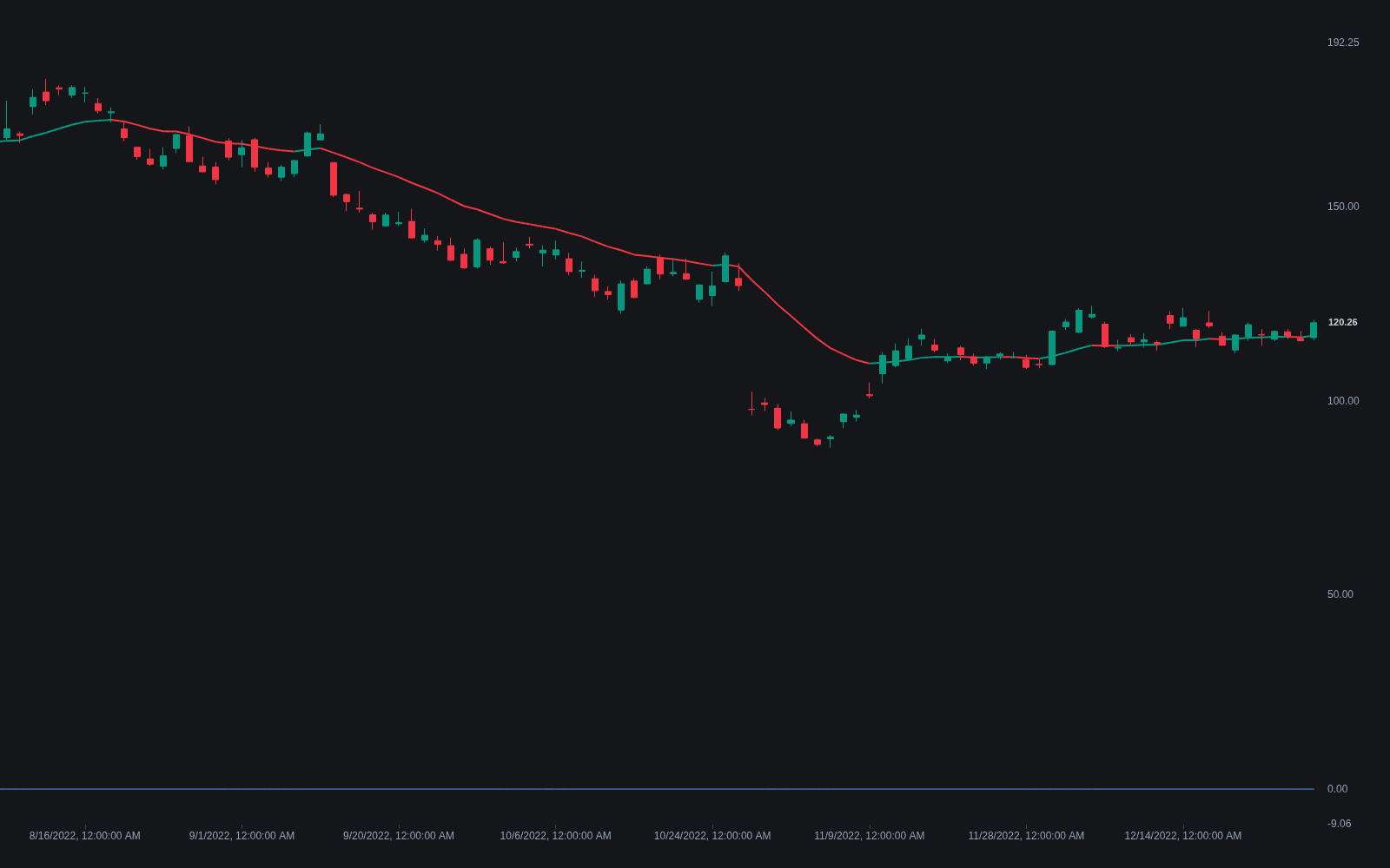
What is a Kalman Filter?

A Kalman filter is a recursive estimator, introduced by Rudolf Kálmán in 1960 for control engineering, that tracks the hidden state of a noisy system one observation at a time. Applied to markets, the usual assumption is that each print is an unobserved 'true' level plus noise. Every bar the filter predicts where that level should be from a simple motion model, then blends the prediction with the new price. The blending weight, called the Kalman gain, is recomputed each step from two variances: how much the true state is allowed to wander (process noise) and how noisy observations are (measurement noise).

Traders use it as an adaptive smoother: when the settings imply prices are informative, the gain rises and the filter hugs price; when they imply noise, it flattens and rides out chop. The same recursion can estimate an evolving hedge ratio between two instruments in pairs trading, an example of adaptive parameterization done with explicit statistics. The caveat is that the output is only as good as the assumed model: the filter still lags at genuine turning points, and badly chosen noise settings produce smooth, confident-looking lines that are simply wrong.

How a Kalman filter works

The filter is a two-step loop, predict then update, run once per bar.

1. 1Specify the model: choose the state to track (a smoothed price level, often paired with its velocity) and set the two noise variances, process and measurement. Their ratio is the filter's real tuning knob.
2. 2Predict: project the state one bar forward with the motion model (unchanged level, or level plus velocity) and widen its uncertainty by the process noise.
3. 3Update: when the bar arrives, compute the Kalman gain from the predicted uncertainty relative to measurement noise, then pull the prediction toward the observed price by that fraction and shrink the uncertainty.
4. 4Repeat every bar. The output plots like a moving average whose responsiveness follows the noise settings; two-state versions also emit a velocity estimate that reads as trend slope.

How it's calculated

A recursively updated price estimate that blends each bar's prediction with the newly observed price, weighted by their relative uncertainties.

This is the scalar random-walk form (state transition and observation both equal to 1) used by chart implementations; the general filter runs the same predict and update cycle with state vectors and covariance matrices.

Only the ratio Q / R matters in steady state: raise it for a faster, noisier estimate, lower it for a smoother, laggier one.

Initialize Est_0 to the first price and Var_0 to any positive value; the gain converges to its steady state regardless.

How traders use it

• As an adaptive baseline: the filtered level serves the familiar moving-average roles (slope color, crossovers, a trailing reference) with responsiveness governed by the noise model rather than a fixed length setting.
• As a dynamic hedge ratio: modeling the regression slope between two assets as the state lets the ratio update bar by bar, replacing a fixed-window linear regression in spread construction.
• As a velocity gauge: constant-velocity variants expose the estimated rate of change directly, which some systems use as a trend/chop classifier or a momentum input.
• As pre-processing: filtering a noisy series before it feeds another indicator trades a little delay for fewer whipsaw flips downstream.

Kalman Filter vs related concepts