Top 5 Metrics for Evaluating Trading Strategies

Profit factor, maximum drawdown, Sharpe ratio, win rate, and expectancy answer different questions about a trading strategy. Read them together: a high win rate can accompany large losses, and a profitable backtest can still have an uncomfortable equity decline.
LuxAlgo combines native charts with Quant, our coding agent, to help turn explicit rules into strategies you can inspect and backtest. The useful next step is understanding what the numbers measure, which assumptions produced them, and what they cannot establish about future trading.
| Metric | Main question | Important limitation |
|---|---|---|
| Profit factor | How large were winning-trade profits relative to losing-trade losses? | Hides trade order and depends on the cost convention. |
| Maximum drawdown | What was the largest observed equity decline from a prior peak? | Historical drawdown is not a ceiling on future losses. |
| Sharpe ratio | How large were average excess returns relative to their variability? | Depends on return frequency, benchmark, and annualization assumptions. |
| Win rate | What fraction of closed trades finished profitable? | Ignores the size of wins and losses. |
| Expectancy | What was the average result per trade? | A sample average is not a promised future outcome. |
There is no universal pass mark such as profit factor above 1.75, drawdown below 20%, or win rate above 50%. Evaluate the strategy's objective, exposure, costs, sample, and alternatives before deciding whether its results are useful.
1. Profit factor: measuring profitability
Profit factor = sum of winning-trade profits ÷ absolute sum of losing-trade losses. If wins total 10,000 and losses total 5,000, profit factor is 2.0: two units won for each unit lost in the measured sample. It is not a 200% return on the account.
TradingView's definition uses realized trade results and excludes open positions. When comparing reports, confirm whether trade P&L includes commissions and other charges, and whether partial exits count as separate trades. A large open loss can coexist with an attractive closed-trade profit factor.
- Below 1: Included losses exceed included profits.
- Exactly 1: Those profits and losses balance under the stated accounting.
- Above 1: Included profits exceed included losses; this alone does not establish robustness.
- No losing trades: The denominator is zero. Treat an infinite or unavailable reading as an edge case, not a superior strategy score.
A very high value may come from a small sample or one exceptional winner. Compare the full result with a sensitivity check that removes the largest winner, clearly labeling that altered sample. Also inspect different chronological periods rather than selecting only the best one.
2. Maximum drawdown: assessing the equity path
At each observation, compare equity with its highest previous value. For positive peak equity, percentage drawdown is (prior peak − current equity) ÷ prior peak × 100. Maximum drawdown is the largest such percentage over the measured period. The worst decline can be ongoing at the end; recovery is not required for it to count.
An account that peaks at 100,000 and declines to 70,000 has a 30% drawdown. It then needs a 30,000 gain on the remaining 70,000, or 42.9%, to return to that peak. A 50% drawdown requires a 100% gain. In general, recovery from a fractional loss d requires d ÷ (1 − d), assuming no deposits or withdrawals.
Check how equity is measured
Closed-trade balance, end-of-day marked equity, and intrabar equity can produce different drawdowns. A strategy that holds losing positions for long periods may look smoother when unrealized losses are omitted. Record sampling frequency and whether open positions are marked to market. Account cash flows also need explicit treatment so deposits are not mistaken for trading gains.
Drawdown duration matters alongside depth. Two strategies can both lose 15% from a peak while taking very different lengths of time to recover. Report the dates of the decline and recovery, or state that recovery has not occurred.
Position size, leverage, and simultaneous exposures influence the equity path. A planned loss budget is different from capital exposure: committing 5,000 to a position does not mean only 5,000 multiplied by a chosen risk percentage can be lost. Correlated positions can decline together, and stop orders do not guarantee execution at the stop price.
3. Sharpe ratio: comparing excess return and variability
For a return series, calculate the strategy return minus the chosen benchmark return for each matching period. The historical Sharpe ratio is the mean of those excess returns divided by their standard deviation. William Sharpe's explanation also describes why the measurement period and time dependence matter.
If mean annual return is 10%, the constant annual risk-free benchmark is 2%, and annual return standard deviation is 5%, the ratio is (10% − 2%) ÷ 5% = 1.6. These inputs must describe compatible periods and a consistent return calculation; do not substitute a cumulative return or mix an annual yield with monthly volatility.
A common annualization multiplies a periodic Sharpe by the square root of periods per year—for example, √12 for monthly returns. That conversion relies on assumptions about return dependence and aggregation. Serial correlation can make it misleading.
Use regularly spaced account returns with cash-flow adjustments, not an arbitrary list of unequal-duration trade profits. State the currency, benchmark, sampling frequency, cost treatment, and whether the figure is annualized. A zero estimated standard deviation makes the ratio undefined. No single cutoff proves that a strategy has an edge.
Sharpe also does not describe every kind of loss risk. Compare it with the equity path, concentrated exposures, and adverse scenarios, especially when a strategy earns many small gains but occasionally suffers a large loss.
4. Win rate: counting profitable trades
Win rate = profitable closed trades ÷ all closed trades × 100. Sixty winners out of 100 closed trades gives 60%. State how breakeven trades and partial exits are counted. A trade that is positive before fees but negative afterward is not a net winner.
Win rate needs payoff size beside it. In one hypothetical sample, 40 winners averaging 200 and 60 losers averaging 100 produce 8,000 − 6,000 = 2,000 across 100 trades, despite a 40% win rate. In another, 70 winners averaging 50 and 30 losers averaging 150 produce 3,500 − 4,500 = −1,000 despite a 70% win rate. Assume each amount already includes costs.
Neither a strategy label such as trend following nor a large historical win percentage supplies a reliable benchmark by itself. Check the actual sample. Moving targets closer can increase the frequency of wins while reducing their size; holding losers longer can make closed-trade statistics look better while hiding open risk.
5. Expectancy: measuring average trade outcome
For a historical sample, expectancy = total net closed-trade P&L ÷ number of closed trades. With win and loss frequencies expressed as fractions, the equivalent form is (win frequency × average win) − (loss frequency × average loss magnitude). Breakeven trades contribute zero but remain in the total count.
Using the original illustrative inputs—55% winners averaging €120 and 45% losers averaging €80—the calculation is (0.55 × €120) − (0.45 × €80) = €30 per trade. If these amounts are net of costs, that is the net sample average. If costs have not been included, deduct them consistently before interpreting the result.
There is no universal “strong” expectancy of €20 or any other cash amount. Monetary expectancy depends on size, instrument value, and currency. It estimates the observed sample; it does not mean each future trade should earn that amount or that the next 100 trades will reproduce it.
One sample connects three metrics
For 100 hypothetical trades with 55 wins of €120 and 45 losses of €80, all net of costs:
| Measure | Calculation | Result |
|---|---|---|
| Win rate | 55 ÷ 100 | 55% |
| Total winning P&L | 55 × €120 | €6,600 |
| Total loss magnitude | 45 × €80 | €3,600 |
| Profit factor | €6,600 ÷ €3,600 | 1.83 |
| Net P&L | €6,600 − €3,600 | €3,000 |
| Expectancy | €3,000 ÷ 100 | €30 per trade |
Those totals do not tell you maximum drawdown: the order and timing of results matter. They also do not provide a Sharpe ratio without a suitable account-return series. One hundred trades is an example count, not a guarantee of statistical reliability; clustered trades can contain much less independent information than the count suggests.
If comparing differently sized trades, consider an additional result in units of initial planned risk, often called R. Compute each trade's net P&L divided by its own recorded initial risk and then average those values. Do not divide average profit by average risk and assume it is the same calculation. Cash expectancy and average R answer different questions.
Review strategy results in LuxAlgo
Ask Quant to implement explicit entry, exit, and sizing rules, review the generated code, and run it on the intended chart. Configure capital, order size, commission, slippage, and other relevant simulation properties. Code that executes successfully still needs checks against the intended trading rules.
The native strategy report shows net profit, closed-trade count, win rate, maximum drawdown, and profit factor in its summary. Its full viewer has Performance, Trades Analysis, and Trades Log tabs. Inspect the equity result, distribution of outcomes, and individual entries and exits rather than selecting a strategy from one headline number.
Do not assume Sharpe and expectancy appear in every summary, or that native Quant supplies automatic alerts when either Sharpe or drawdown crosses a limit. Calculate any additional metric from an appropriate, reconciled dataset. Changing a chart timeframe reruns the strategy on different bars; it is not the same as changing the sampling frequency of an unchanged equity series.
Save the run so the script, symbol, timeframe, inputs, and properties remain reproducible. Use standard tradable candle prices for evaluation; synthetic Heikin Ashi prices can distort simulated fills. Compare variants on the same dates and assumptions before extending the test to other markets.
Separate backtests from trading records
The LuxAlgo Journal is a separate account-level record for manual, imported, or supported broker-synced fills. It derives closed round trips from fills, including fees, net P&L, and win/loss/breakeven status. Reconcile duplicates, missing executions, and account selection before comparing those records with a strategy simulation.
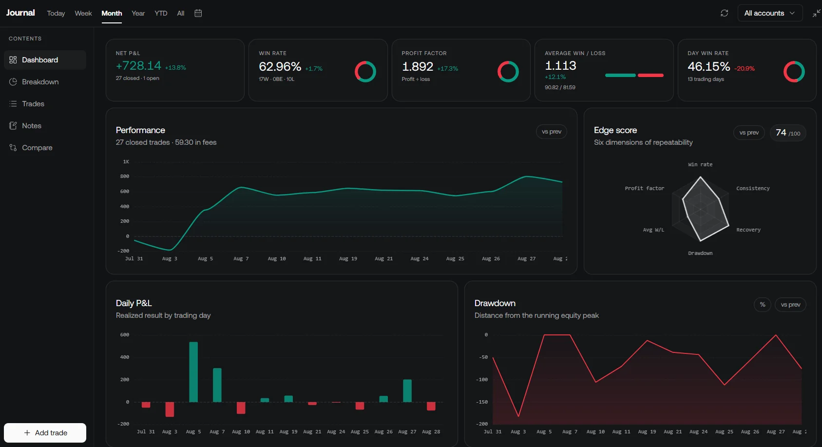
Build a repeatable review process
- After each session: Reconcile executions, fees, open positions, and deviations from the rules.
- At a planned weekly review: Inspect recent performance, concentrations, unusually large trades, and data problems without rewriting rules after every loss.
- At a broader periodic review: Compare the frozen strategy with a relevant benchmark and reserved later data. Record changes as new versions.
Include the testing period, number of trades, market exposure, cost assumptions, and selection history with the five metrics. Stress higher costs and less favorable execution. A review schedule helps organize evidence; it does not ensure that a strategy remains profitable.
FAQs
How to evaluate a trading strategy?
Define the rules and accounting assumptions, then review profit factor, maximum drawdown, Sharpe ratio, win rate, and expectancy together. Reconcile costs and individual trades, inspect open-position risk and the equity path, compare a relevant baseline, and test fixed rules on later data. No universal metric threshold or trade count proves future profitability.
Read next