Historical Volatility: Calculating Volatility Using Past Prices

By Jacob DenbrockOct 20, 202514 min readReviewed by Christopher Downie on Sep 10, 2026

Historical volatility is the annualized standard deviation of an asset's past returns: a single percentage that says how much the price actually moved over a chosen window, with no opinion about direction. The standard form takes the natural log of each close divided by the previous close, measures the dispersion of those returns over a lookback, and multiplies by the square root of the number of periods in a year, so a daily figure of 1.15% becomes an annualized 18%. It is backward-looking by construction, which is both its virtue and its limit: it reports what happened, it can be reproduced by anyone with the same closes, and it says nothing about the next shock. Its practical value is comparison. Expressed in volatility units, a quiet blue chip and a wild crypto pair sit on one scale, which is what position sizing, regime filters and the comparison with option-implied volatility all exploit.

Key points:

Four steps: log returns, standard deviation over a window, annualize by the square root of periods per year, quote as a percentage.
The window and the divisor matter: a 10-bar and a 30-bar figure tell different stories, and sample versus population standard deviation changes the number by a few percent.
Read it against its own history: normal levels differ across markets, so a percentile of the same symbol's past readings beats any fixed threshold.
Volatility clusters: elevated readings tend to follow elevated readings, so the current level is informative about near-term movement even though it forecasts nothing about direction.

The LuxAlgo Historical Volatility indicator is the standard close-to-close calculation with a published source, and it opens on Quant Charts in one click. Quant, our coding agent, can turn a volatility-sized rule into a strategy you can inspect in Code and test with Run.

Historical Volatility: Video Overview

The Options Industry Council published this overview in August 2025. It frames historical volatility from the options trader's side, as the realized figure against which implied volatility is judged.

How to Calculate Historical Volatility Step by Step

The Library's close-to-close historical volatility page calls this the oldest and most widely quoted volatility estimator and the default meaning of the term. It needs nothing but closing prices, and the only real decisions are the lookback window and the annualization factor.

Collect Closing Prices

Gather daily closes for one more bar than the window you want: 11 closes for 10 returns, 21 for 20, 31 for 30. Ten to thirty daily returns are the common charting windows; the native indicator defaults to 10, and 20 and 30 are frequent choices in options work. Longer windows, out to a year of data, are steadier and suit portfolio risk budgeting; Karthik Rangappa of Zerodha Varsity notes that six months of data is workable and that he prefers a full year. Shorter windows track the current regime closely but jump on every large return. Use the same session convention throughout: a 24-hour feed and a regular-hours feed give different closes on futures and forex.

Calculate Log Returns

For each bar, the return is ln(Close today ÷ Close yesterday). If a stock closed at $180.50 and then $182.75, the log return is ln(182.75 ÷ 180.50) = 0.01239, about 1.24%. Log returns are used rather than simple percentage changes because they add across periods, which is what makes the square-root-of-time annualization exact, and because they are the convention behind every published volatility figure, so the result lines up with quoted numbers. In a spreadsheet, with closes in column B starting at B2, the formula in C3 is =LN(B3/B2), copied down.

Take the Standard Deviation and Annualize

Compute the standard deviation of the returns over the window, then multiply by the square root of the periods per year: √252 = 15.875 for daily bars on markets with roughly 252 trading days, √365 is often used for markets that trade every day, √52 for weekly bars and √12 for monthly. Multiply by 100 to quote a percentage. The sample form, =STDEV.S in a spreadsheet, divides by n − 1 and is what the native indicator uses; many charting platforms use the population divisor n, which gives a slightly lower number on the same data. Some implementations also assume a zero mean rather than subtracting the window's average return, which matters little on daily data. Check which convention a source uses before comparing its figures with yours.

The table runs the full calculation on eleven hypothetical closes, the native indicator's 10-return window.

Day	Close	Log return	Return − mean	Squared
0	$100.00	—	—	—
1	$101.20	+1.193%	+0.781%	0.0000611
2	$100.40	−0.794%	−1.205%	0.0001452
3	$102.10	+1.679%	+1.268%	0.0001607
4	$103.00	+0.878%	+0.466%	0.0000217
5	$101.80	−1.172%	−1.583%	0.0002507
6	$102.60	+0.783%	+0.371%	0.0000138
7	$104.10	+1.451%	+1.040%	0.0001082
8	$103.30	−0.771%	−1.183%	0.0001399
9	$105.00	+1.632%	+1.221%	0.0001491
10	$104.20	−0.765%	−1.176%	0.0001384
Result	Mean return 0.411%; sample standard deviation 1.149% per day; × 15.875 = 18.2% annualized (population divisor: 1.090% and 17.3%)

An 18% annualized reading means a one-standard-deviation move over a year of about 18%, or about 1.15% on a typical day, under the assumption that daily returns are independent. That assumption is an approximation, and real returns have fatter tails than the normal curve, so treat the annualized figure as a shared yardstick rather than a probability statement. Notice too what happens when a single large return enters or leaves a short window: the figure leaps as it arrives and steps back down when it ages out, even though nothing happened on that later bar.

Reading and Using Historical Volatility

LuxAlgo Historical Volatility on Quant Charts plotted as an annualized percentage line in a pane below a candlestick chart — The LuxAlgo Historical Volatility indicator on Quant Charts, from the Library preview. The line reads directly as an annualized percentage; the default window is 10 bars.

Regimes: Read It Against Its Own History

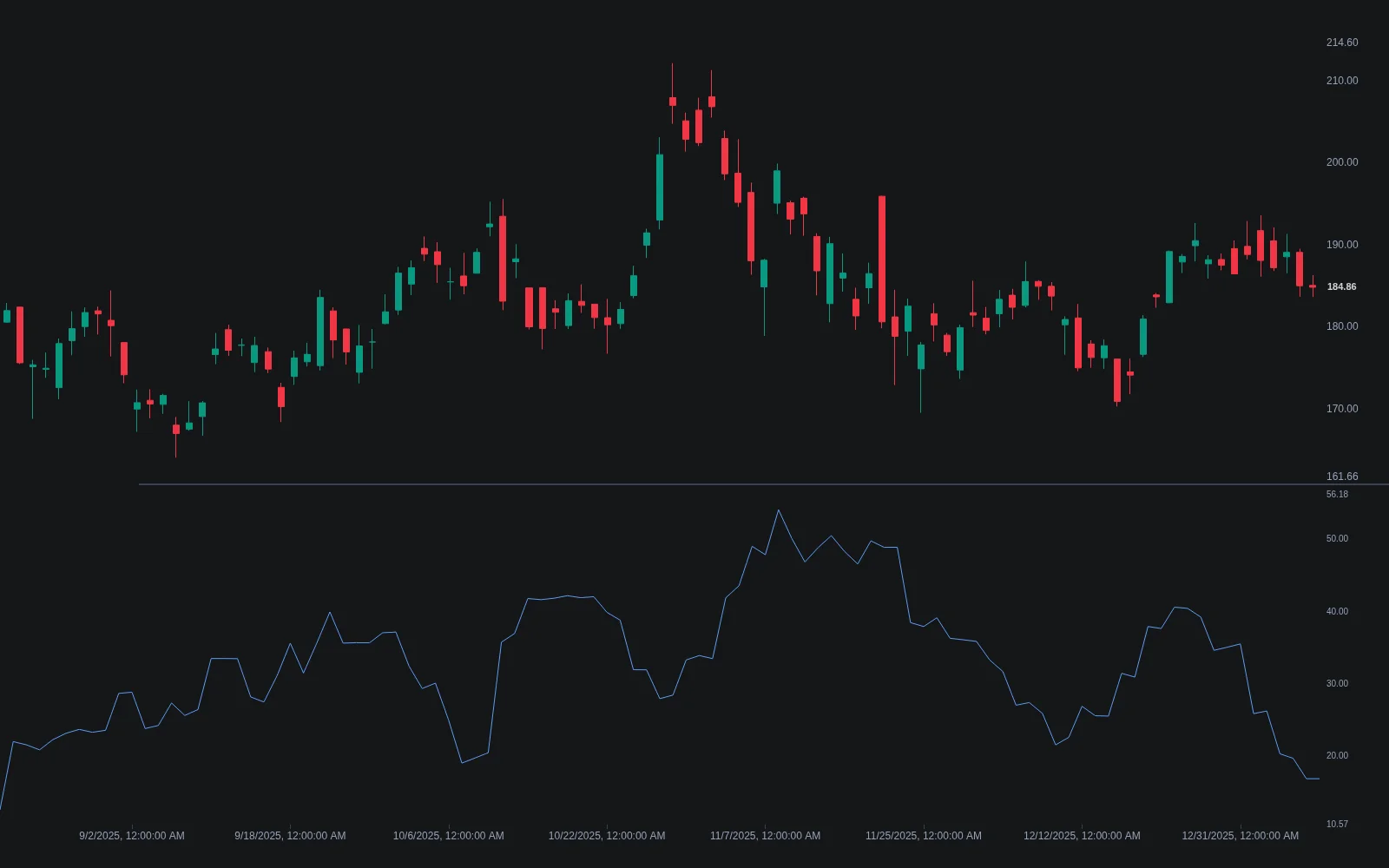
The reading is direction-blind and its normal level differs by market: 15% is ordinary for an equity index and extraordinary for a stablecoin. So the useful comparison is with the same symbol's past, a volatility percentile or rank over the last year, for instance. A low percentile marks a quiet regime, and long compressions often precede expansion; a high percentile marks an active regime in which stops need to be wider and sizes smaller to keep risk per trade comparable. Because volatility is persistent, a spike is a regime statement rather than a one-bar event, and the reading tends to stay elevated for a while after it. A cross-check against ATR is worth the second pane: ATR includes intrabar travel that close-to-close returns ignore, while historical volatility captures overnight gaps that a range measure can understate, and disagreement between the two is itself information.

Position Sizing

The most concrete use is volatility-targeted sizing: divide a fixed risk budget by the instrument's current volatility so that a typical move produces a similar equity impact in every market. Consider a $25,000 account with a budget of $250, 1%, for a one-standard-deviation daily move. Dividing the annualized figure by 15.875 gives the daily figure; dividing the budget by that gives the position.

Instrument	Annualized HV	Daily one-sigma move	Position for a $250 one-sigma budget	Share of $25,000
Index ETF	15%	0.94%	$26,458	106%, capped at the concentration limit
Quiet large cap	18%	1.13%	$22,048	88%, capped at the concentration limit
Volatile growth stock	55%	3.46%	$7,216	29%
Crypto pair	80%	5.04%	$4,961	20%

Two lessons sit in that table. Volatility sizing shrinks exposure in wild instruments and expands it in quiet ones, which is the point, but on the quiet end it will happily ask for more than the account, so a concentration cap has to sit on top of it. And the sizing is only as current as the estimate: when volatility jumps faster than a 10-bar window updates, the position sized for last week's tape takes this week's larger moves, and the realized loss can exceed the budget. Volatility targeting standardizes an estimate of risk; it does not cap the outcome. For a per-trade stop the same arithmetic applies: a $50 stock at 32% annualized has a daily one-sigma move of about $1.01, so a two-sigma stop sits about $2.02 away and a $250 risk budget buys 124 shares. See Risking It Right for the budgeting logic.

Options: Realized Versus Implied

Option pricing models such as Black-Scholes take a volatility input, and the volatility that makes a model's price match the market's price is the implied volatility. Historical volatility is the measured leg of the comparison. When options price substantially more volatility than the underlying has been realizing, sellers of premium see a cushion and buyers face a headwind; when implied sits below realized, the reverse. That spread is tracked as the volatility risk premium, and it is usually positive, because the options market charges for the risk that realized volatility jumps. A 30-day historical figure of 25% against an at-the-money implied of 35% therefore says the options are rich relative to recent movement, not that they are mispriced; the market may be pricing an event the last 30 days did not contain. Implied volatility rank and percentile normalize the implied side the same way a percentile normalizes the realized side.

Two Estimators, Same Stock

The choice of window changes the picture more than beginners expect. Suppose a stock has had a calm two months and then one 8% earnings day. A 10-day figure that includes the earnings bar might read 45% annualized while a 60-day figure reads 24%; a week later, once the bar ages out of the short window, the 10-day figure could drop below 15% while the 60-day figure still carries the shock. Neither is wrong. The short window describes the current tape, the long one the recent history, and a rule that sizes off the short window will swing its positions far more than one sized off the long. Record the window with every number you publish or test.

Historical Volatility on Quant Charts

TSLA candlestick chart in TradingView with LuxAlgo Price Action Concepts structure labels and volume-tagged order blocks, and a volatility line in the pane below — A TSLA chart in TradingView with LuxAlgo Price Action Concepts structure labels and order blocks, and a volatility line in the pane below. The toolkit overlays come from their own structure logic and do not compute historical volatility.

The Native Historical Volatility

The Library's Historical Volatility is the standard raw close-to-close calculation: each bar's log return feeds a sample standard deviation over a window of Length 10 by default, scaled by the square root of Periods Per Year (252, with 52 for weekly and 12 for monthly bars) when Annualize is on, and plotted as a single percentage line. The source is published on the page, so the n − 1 divisor and the mean subtraction can be checked directly. There are no signal alerts, deliberately: the indicator is a measurement, and thresholds belong to the symbol's own history rather than to fixed levels.

Tool	What it adds	Where it runs
Historical Volatility	Annualized standard deviation of close-to-close log returns	Quant Charts, from the Library page
Standard Deviation	Raw price dispersion over a window, the same statistic applied to closes	Quant Charts, from the Library page
Average True Range	Range-based volatility in price units, including intrabar travel; the natural stop-distance measure	Quant Charts, from the Library page
Bollinger Bands	Standard deviation applied as a band width around a moving average	Quant Charts, from the Library page
Keltner Channels	ATR-based channel, a range-based counterpart to the bands	Quant Charts, from the Library page
Price Action Concepts, Signals & Overlays, Oscillator Matrix	LuxAlgo toolkits with their own structure, signal and momentum logic	TradingView; none of them computes historical volatility

Testing a Volatility-Sized Rule with Quant

Write the rule completely: the entry and exit logic, the volatility window and divisor, the annualization basis, the risk budget, how the position size is derived from the current reading, the concentration cap, and how often the size is recomputed. Describe it to Quant, inspect the Code to confirm the volatility is computed from completed bars and the size is set at entry rather than drifting with every tick, and click Run. The Making Strategies with Quant guide shows the workflow, and the native backtest guide explains the Backtest Summary: net profit, trade count, win rate, maximum drawdown and profit factor, with commission and slippage set in the strategy properties.

Adding indicators in Quant Charts. Historical Volatility and Average True Range can be loaded in separate panes to see where the close-based and range-based measures disagree.

Three comparisons are worth running. The same entry rule with fixed-dollar sizing against volatility-targeted sizing, to see what the sizing does to drawdown and to the distribution of trade outcomes. A 10-bar window against a 30-bar window as the sizing input, to see how much position turnover the short window creates. And a volatility-percentile filter, trading only when the reading sits below its 50th percentile for breakouts or above it for mean reversion, against no filter. Read maximum drawdown and trade count before headline return, and hold out data the window choice never saw. LuxAlgo's Price Action Concepts, Signals & Overlays and Oscillator Matrix toolkits run on TradingView with their own calculations; none of them computes historical volatility, and a toolkit signal in a low-volatility regime is confluence to test rather than confirmation. The legacy Backtesting Assistant is a separate product with its own workflow and is not needed for these tests, and no LuxAlgo tool places orders at a broker.

Strengths and Limitations

Aspect	Strength	Limitation
Inputs	Needs only closes; reproducible by anyone with the same data	Discards everything price did inside the bar; range-based estimators such as Parkinson or Yang-Zhang use more of each bar
Timing	Captures overnight gaps, since each return spans them	Lags by construction; a shock enters the window late and leaves it abruptly
Comparability	Puts different instruments on one annualized scale	Normal levels still differ by market, so thresholds must be relative
Statistics	The convention behind quoted volatility and option models	Square-root-of-time scaling assumes independent, normal-ish returns; real returns are fat-tailed and cluster
Forecasting	Persistence makes the current level informative about near-term movement	Says nothing about direction and cannot anticipate a regime break; EWMA and GARCH models weight recent returns more heavily for that reason
Sizing	Gives a systematic denominator for risk budgets	Sizes for yesterday's volatility; a fast jump can push losses past the budget

Conclusion

Historical volatility is the simplest honest measure of how much a market has been moving: log returns, a standard deviation, an annualization factor. Its power is comparability, letting one risk budget span quiet and wild instruments and letting realized movement be set against what options imply. Its limits are equally plain: it looks backward, it treats every return in the window equally, and it knows nothing about direction or the next shock. Used as a yardstick against a symbol's own history, and as a sizing denominator under a concentration cap, it is one of the few indicators that improves almost any rule it is attached to. Used as a forecast, it disappoints exactly when it matters.

Key Takeaways

Four steps, two choices. Log returns, standard deviation, annualize, quote as a percentage; the window and the divisor are the decisions that change the number.
Relative, not absolute. Compare a reading with the same symbol's past through a percentile, never with a fixed threshold.
Size with it, cap it. Volatility-targeted sizing evens risk across markets but must sit under a concentration limit and will lag a fast regime change.
Realized versus implied. The spread between historical and implied volatility is what option traders actually trade; the historical figure is the measured leg.
Native and testable. The Historical Volatility indicator opens on Quant Charts with a published source, and Quant can build and test a volatility-sized rule against a fixed-size version.

FAQs

How do you calculate historical volatility?

Take the natural log of each close divided by the previous close, compute the standard deviation of those returns over a window such as 10, 20 or 30 bars, multiply by the square root of the periods per year (√252 for daily equity data) and by 100. A daily standard deviation of 1.15% becomes about 18% annualized.

What is the difference between historical and implied volatility?

Historical volatility measures how much the underlying actually moved over a past window. Implied volatility is the volatility number that makes an option-pricing model's price match the option's market price, so it is the movement the options market is currently paying for. The gap between them, the volatility risk premium, is usually positive.

Why use log returns instead of percentage changes?

Log returns add cleanly across periods, which is what makes multiplying by the square root of time exact, and they are the convention behind every published volatility figure, so the result matches quoted numbers. On daily data the difference from simple returns is small; on large moves it is not.

Should I use the sample or population standard deviation?

The sample form divides by n − 1 and is what statistics texts and the native Historical Volatility indicator use; many charting platforms divide by n. On a 10-bar window the sample figure is about 5% higher than the population figure on the same data. Either is fine as long as you compare like with like.

How do I use historical volatility for position sizing?

Divide the annualized figure by the square root of the periods per year to get a one-period move, then divide your risk budget by that move to get a position size. A $250 budget against a 3.46% daily move gives about $7,200 of exposure. Add a concentration cap, because quiet instruments will otherwise be sized beyond the account.

Can I plot and backtest historical volatility on Quant Charts?

Yes. Open the Historical Volatility indicator from the Library with Open on Quant Charts; Length, Annualize and Periods Per Year are the inputs. To test a volatility-sized or volatility-filtered rule, describe the entry logic, the window, the budget and the sizing formula to Quant, inspect the Code and click Run.