SQL for Trading: Unlock Financial Data
SQL is the language of the data layer under a trading operation: the place where years of candles, fills and reference data are stored once, cleaned once and queried by everything else. It is not an execution engine and it will not place an order, but a trader who can write window functions can compute returns, moving averages, RSI and VWAP over millions of rows in a few lines, generate signals without lookahead, and run an honest first backtest before any Python or Pine Script exists. This guide covers choosing a database, designing a candle schema that will not corrupt your prices, the window-function queries that do the analytical work, a backtest that fills on the next bar and pays commission, the pitfalls that make SQL backtests lie, and how the database connects to Python, MetaTrader and charting tools. It closes with where Quant Charts fits: the chart is where a rule gets tested visually and quickly, with Quant, our coding agent, writing the Pine Script, and SQL is where the research data behind it lives.
Key points:
- Window functions are the whole trick. LAG, LEAD, AVG OVER and SUM OVER turn a candle table into returns, indicators, signals and equity curves without leaving the database.
- Store prices as exact decimals and times in UTC. NUMERIC for prices, BIGINT for volume, a composite key on symbol and timestamp, and partitions by month once the table is large.
- Backtest on the next bar. A signal computed on a bar's close is held from the next bar; the LAG of the signal, not the signal itself, is the position.
- Pick the engine for the job. DuckDB or SQLite for a research laptop, PostgreSQL with TimescaleDB for a shared store, ClickHouse or QuestDB for tick-level scale.
Choosing a Database
Every serious SQL engine supports the window functions this article relies on, so the choice is about where the data lives and how much of it there is, not about syntax.
| Engine | Best for | Notes |
|---|---|---|
| DuckDB | Research on a laptop; querying Parquet and CSV files directly | Embedded, columnar, fast analytics; works inside Python with no server to run |
| SQLite | Portable single-file stores; MetaTrader 5's built-in database | Window functions supported; ideal for small bots and local journals |
| PostgreSQL, with TimescaleDB | A shared, durable store for a team or several systems | Rich SQL, partitioning, extensions; TimescaleDB adds time-series compression and continuous aggregates |
| ClickHouse, QuestDB | Tick data and order-book history at scale | Columnar time-series engines built for billions of rows and fast range scans |
| Microsoft SQL Server, Azure SQL | Enterprises already standardised on it | Full window-function support via the OVER clause; T-SQL date functions differ from the standard |
The examples below use standard SQL that runs on PostgreSQL and DuckDB; where a function differs on SQL Server or SQLite the difference is noted.
A Candle Schema That Stays Correct
Three decisions prevent most data problems. Prices are stored as NUMERIC, never as FLOAT, because binary floating point cannot represent most decimal prices and the errors accumulate in sums. Timestamps are stored in UTC with the exchange time zone recorded on the instrument, because daylight-saving rules have ruined more backtests than bad strategies have. And the primary key is the pair of symbol and timestamp, which makes duplicate loads impossible by construction.
CREATE TABLE instruments (
    symbol        TEXT PRIMARY KEY,
    exchange      TEXT NOT NULL,
    tick_size     NUMERIC(18, 8) NOT NULL,
    exchange_tz   TEXT NOT NULL              -- e.g. 'America/New_York'
);

CREATE TABLE candles (
    symbol        TEXT NOT NULL REFERENCES instruments(symbol),
    ts            TIMESTAMPTZ NOT NULL,     -- bar open time, stored in UTC
    open          NUMERIC(18, 8) NOT NULL,
    high          NUMERIC(18, 8) NOT NULL,
    low           NUMERIC(18, 8) NOT NULL,
    close         NUMERIC(18, 8) NOT NULL,
    volume        BIGINT NOT NULL CHECK (volume >= 0),
    PRIMARY KEY (symbol, ts),
    CHECK (low <= open AND low <= close AND high >= open AND high >= close)
);

-- Most queries are one symbol over a time range; the primary key already serves them.
-- Add a time-only index for cross-sectional queries such as "all symbols on a date".
CREATE INDEX candles_ts_idx ON candles (ts);
Once the table passes a few hundred million rows, partition it by month (PostgreSQL's declarative partitioning or a TimescaleDB hypertable) so that range scans touch only the partitions they need and old data can be compressed or dropped as a unit. Keep a separate table of corporate actions and a view of adjusted prices rather than overwriting raw closes; a backtest that cannot be reproduced because the data changed underneath it is not a backtest.
Returns and Moving Averages
Window functions compute a value for each row using its neighbours without collapsing the rows, which is exactly the shape of time-series analysis. LAG reaches back a bar, AVG OVER a frame computes a rolling mean, and PARTITION BY keeps each symbol's calculation separate.
-- Daily returns per symbol; NULLIF guards against a zero previous close.
SELECT
    symbol,
    ts,
    close,
    close - LAG(close) OVER w                                   AS change_abs,
    close / NULLIF(LAG(close) OVER w, 0) - 1                    AS return_simple
FROM candles
WHERE ts >= TIMESTAMPTZ '2024-01-01'
WINDOW w AS (PARTITION BY symbol ORDER BY ts)
ORDER BY symbol, ts;
-- 20- and 50-bar simple moving averages that are NULL until the window is full.
SELECT
symbol,
ts,
close,
CASE WHEN COUNT(*) OVER w20 = 20
THEN AVG(close) OVER w20 END AS sma_20,
CASE WHEN COUNT(*) OVER w50 = 50
THEN AVG(close) OVER w50 END AS sma_50
FROM candles
WINDOW
w20 AS (PARTITION BY symbol ORDER BY ts ROWS BETWEEN 19 PRECEDING AND CURRENT ROW),
w50 AS (PARTITION BY symbol ORDER BY ts ROWS BETWEEN 49 PRECEDING AND CURRENT ROW);The COUNT guard matters. Without it the first nineteen rows of a 20-bar average are averages of fewer bars, which look like data and are not. SQL Server does not support the WINDOW clause; repeat the OVER definition inline instead. SQLite supports both.
RSI and VWAP
RSI compares average gains to average losses over a lookback. Wilder's original uses a recursive smoothing that needs a recursive CTE or a procedural loop in SQL; the simple-average variant, often called Cutler's RSI, is a straightforward window query and is what most SQL implementations actually compute. State which one you use, because the two differ.
-- 14-bar RSI with simple averages (Cutler's RSI).
WITH changes AS (
    SELECT symbol, ts, close,
           close - LAG(close) OVER (PARTITION BY symbol ORDER BY ts) AS chg
    FROM candles
), gl AS (
    SELECT symbol, ts, close,
           CASE WHEN chg > 0 THEN chg  ELSE 0 END AS gain,
           CASE WHEN chg < 0 THEN -chg ELSE 0 END AS loss
    FROM changes
    WHERE chg IS NOT NULL                       -- the first bar has no change
), avgs AS (
    SELECT symbol, ts, close,
           AVG(gain) OVER w AS avg_gain,
           AVG(loss) OVER w AS avg_loss,
           COUNT(*)  OVER w AS n
    FROM gl
    WINDOW w AS (PARTITION BY symbol ORDER BY ts ROWS BETWEEN 13 PRECEDING AND CURRENT ROW)
)
SELECT symbol, ts, close,
       CASE WHEN n < 14 THEN NULL
            WHEN avg_loss = 0 THEN 100
            ELSE 100 - 100 / (1 + avg_gain / avg_loss) END AS rsi_14
FROM avgs;
-- Session VWAP: cumulative price x volume over cumulative volume, reset each trading day.
SELECT
symbol,
ts,
close,
SUM((high + low + close) / 3 * volume) OVER s
/ NULLIF(SUM(volume) OVER s, 0) AS vwap
FROM candles
WINDOW s AS (
PARTITION BY symbol, (ts AT TIME ZONE 'America/New_York')::date
ORDER BY ts
ROWS BETWEEN UNBOUNDED PRECEDING AND CURRENT ROW
);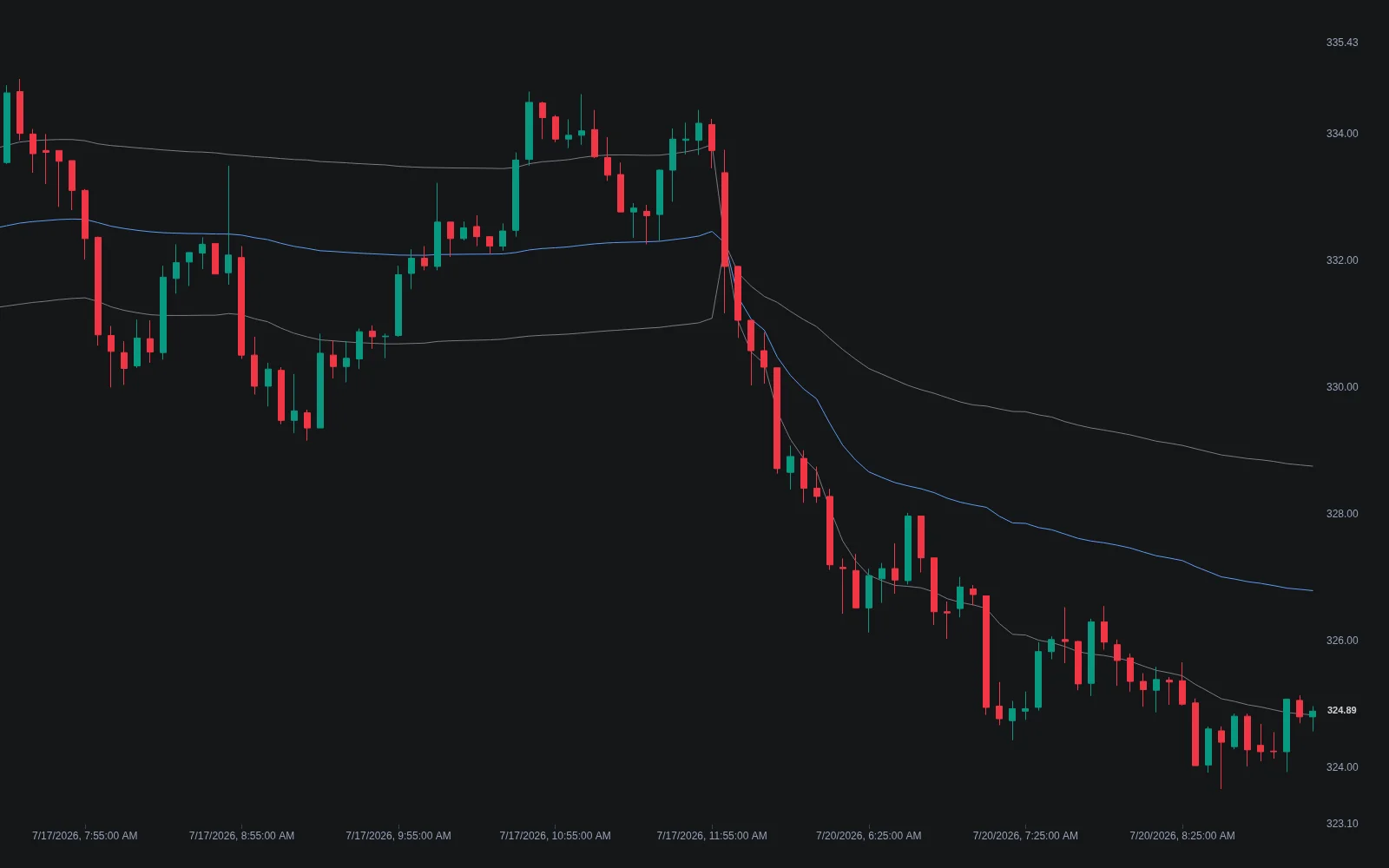
The session partition uses the exchange's local date, which is why the schema records the time zone. On SQL Server, replace the AT TIME ZONE cast with the T-SQL equivalent; on SQLite, store the session date as a column at load time.
Signals and an Honest Backtest
A crossover signal is a comparison between this bar's averages and the previous bar's, so it is two LAGs. The mistake to avoid is treating the bar on which the signal fires as the bar on which the trade happens. A signal is known at the close; the position it implies exists from the next bar. In SQL that means the position column is the LAG of the signal state, and the return earned on a bar is that lagged position times the bar's return.
WITH ma AS (
    SELECT symbol, ts, close,
           CASE WHEN COUNT(*) OVER w10 = 10 THEN AVG(close) OVER w10 END AS sma_10,
           CASE WHEN COUNT(*) OVER w20 = 20 THEN AVG(close) OVER w20 END AS sma_20
    FROM candles
    WINDOW w10 AS (PARTITION BY symbol ORDER BY ts ROWS BETWEEN 9 PRECEDING AND CURRENT ROW),
           w20 AS (PARTITION BY symbol ORDER BY ts ROWS BETWEEN 19 PRECEDING AND CURRENT ROW)
), state AS (
    -- 1 when the fast average is above the slow one at this bar's close, else 0
    SELECT symbol, ts, close,
           CASE WHEN sma_10 > sma_20 THEN 1 ELSE 0 END AS in_market
    FROM ma
    WHERE sma_20 IS NOT NULL
), positioned AS (
    SELECT symbol, ts, close, in_market,
           LAG(in_market, 1, 0) OVER (PARTITION BY symbol ORDER BY ts) AS position,   -- held from next bar
           close / NULLIF(LAG(close) OVER (PARTITION BY symbol ORDER BY ts), 0) - 1  AS bar_return
    FROM state
), pnl AS (
    SELECT symbol, ts, position, bar_return,
           position * COALESCE(bar_return, 0)
             - ABS(in_market - position) * 0.0005                        AS strat_return   -- 5 bps per change
    FROM positioned
), curve AS (
    SELECT symbol, ts, strat_return,
           EXP(SUM(LN(1 + strat_return)) OVER (PARTITION BY symbol ORDER BY ts)) AS equity
    FROM pnl
)
SELECT symbol,
       COUNT(*)                                        AS bars,
       MAX(equity) FILTER (WHERE ts = last_ts)         AS final_equity,
       MIN(equity / running_peak - 1)                  AS max_drawdown
FROM (
    SELECT *,
           MAX(equity) OVER (PARTITION BY symbol ORDER BY ts) AS running_peak,
           MAX(ts)     OVER (PARTITION BY symbol)             AS last_ts
    FROM curve
) x
GROUP BY symbol;
Read what the query does and does not claim. Trades happen at the next bar's close rather than its open, a simplification that is slightly conservative for a trend rule; a version that fills at the next open needs the open joined in. Commission is charged on every change of position. The equity curve is a product of bar returns computed through logarithms, and drawdown is measured against a running peak on every bar. It quotes no result, because the result depends on your data; the point is that the arithmetic cannot look into the future. Our guide to building a backtesting engine in Python covers what to add when the rule outgrows a single query.
Counting Tests of a Price Level
Support and resistance analysis in SQL is a bucketing problem: round lows to a price band and count how often each band was touched in a period. Bands are defined in ticks so the query works across instruments.
-- Price bands touched by the daily low at least three times in the last 60 sessions.
WITH recent AS (
    SELECT c.symbol, c.ts, c.low, i.tick_size
    FROM candles c JOIN instruments i USING (symbol)
    WHERE c.symbol = 'SPY'
      AND c.ts >= (SELECT MAX(ts) FROM candles WHERE symbol = 'SPY') - INTERVAL '60 days'
), bands AS (
    SELECT symbol, low,
           FLOOR(low / (tick_size * 25)) * (tick_size * 25) AS band_floor   -- 25-tick bands
    FROM recent
)
SELECT symbol, band_floor, COUNT(*) AS touches, MIN(low) AS lowest_low
FROM bands
GROUP BY symbol, band_floor
HAVING COUNT(*) >= 3
ORDER BY touches DESC, band_floor;
Pitfalls That Make SQL Backtests Lie
| Pitfall | How it shows up | Fix |
|---|---|---|
| Lookahead through LEAD | Using LEAD(close) to decide today's trade, or filling on the signal bar | Positions are LAG of the signal; LEAD is only for describing what happened after |
| Partial windows | The first rows of a rolling average are averages of too few bars | Guard with COUNT(*) OVER the same frame, as the SMA query does |
| Float prices | Sums and comparisons drift; two systems disagree on a level | NUMERIC columns; cast to float only for statistics that tolerate it |
| Time-zone drift | Sessions split across dates; daily bars shift around clock changes | Store UTC, record the exchange zone, derive session dates explicitly |
| Survivorship bias | Backtest universe contains only symbols that still exist | Keep delisted instruments and a listing-date table; filter by what was tradable at the time |
| Unadjusted prices | Splits appear as crashes; dividends inflate drawdowns | Raw table plus a corporate-actions table and an adjusted view |
| Invalid SQL copied from the web | HAVING on a window alias, RSI fragments that never finish | Run every query on real data before quoting a result from it |
Connecting SQL to the Rest of the Stack
Python. pandas reads any query result into a DataFrame, and DuckDB goes further: it queries pandas DataFrames, Parquet and CSV files directly with SQL from inside a Python process, which makes it the natural research companion. Heavy aggregation stays in SQL; modelling and plotting happen in Python. Our Python for trading guide covers the other half.
MetaTrader 5. MQL5 includes database functions built on SQLite, so an Expert Advisor can store its own trades and read reference data from a local database file without any external server. This is a local store for a bot, not a shared warehouse; see our MetaTrader backtesting guide for the platform side.
Charting. TradingView's Charting Library, the embeddable product for developers, connects to a datafeed you implement, so a web application can chart data served from your own database. That is a developer integration, not a feature of the retail TradingView site, and it is unrelated to Pine Script.
Java, C# and other services. Every JDBC or ADO.NET driver reads the same tables; the schema above is deliberately plain so that a Java risk service and a Python notebook see identical numbers. Our Java for finance guide covers the JVM side.
Where Quant Charts Fits
SQL is where research data lives; Quant Charts is where a rule is tested on a chart in minutes. The two divide the work cleanly. When a query surfaces a candidate, a crossover that looks promising in the equity curve above, a VWAP behaviour you want to see bar by bar, describe the rule to Quant and it writes the strategy in Pine Script and plots it on the active chart. Open Code to read the logic, click Run, and the Backtest Summary reports net profit, trade count, win rate, maximum drawdown and profit factor with commission and slippage set in the strategy properties, which is the same honesty the SQL backtest enforces, with fills, costs and a visual check included. The Library's VWAP indicator is the chart-side twin of the VWAP query, with session, week and month anchors and deviation bands. The Making Strategies with Quant guide shows the workflow.
Two facts about the data side. Quant Charts uses LuxAlgo market data delivered by a single provider in front of several venues, with no exchange accounts or API keys to connect, so it is not a place to load your own database; it is where you look at the market and test rules against the platform's own history. The Journal records fills from a connected broker or by hand, which is the one dataset worth exporting to SQL for your own decision-versus-fill analysis. One boundary: the LuxAlgo platform does not place orders for you.
Conclusion
SQL earns its place in a trading stack by doing one thing better than anything else: holding the data once, exactly, and answering questions about it fast. Window functions turn that store into returns, indicators, signals and equity curves, and a backtest written with the position as the lag of the signal cannot look into the future. The discipline is the same as in every other language, exact prices, an explicit exchange zone, full windows, next-bar fills and costs on every change, and the payoff is a research layer that every other tool can trust. Test the candidates it produces on Quant Charts, where Quant writes the Pine Script and the Backtest Summary asks the same questions with a chart attached.
Key Takeaways
- Schema first. NUMERIC prices, UTC timestamps with the exchange zone, a symbol-plus-time key, partitions when large.
- Window functions do the analysis. LAG for returns and signals, AVG OVER with a COUNT guard for averages, SUM OVER for VWAP.
- Position is the lag of the signal. Charge commission on every change; build equity with EXP of summed logs; measure drawdown against a running peak.
- Match the engine to the scale. DuckDB and SQLite locally, PostgreSQL with TimescaleDB shared, ClickHouse or QuestDB for ticks.
- Chart the candidates on Quant Charts. Quant writes the Pine Script, Code shows it, Run backtests it; SQL stays the data layer.
FAQs
Why use SQL for trading data instead of spreadsheets or CSV files?
A database stores the data once with constraints that prevent duplicates and bad rows, answers questions over millions of candles in seconds, and gives every tool, Python, Java, a bot, the same numbers. Window functions compute returns, indicators and signals in place, and the query text is a reproducible record of exactly what was calculated.
Which database is best for trading data?
For research on one machine, DuckDB, which queries Parquet and CSV directly and runs inside Python, or SQLite for a portable single file. For a shared store, PostgreSQL, with TimescaleDB for time-series features. For tick-level history at scale, ClickHouse or QuestDB. SQL Server and Azure SQL are sensible where a firm already runs them. All support the window functions used here.
How do I calculate a moving average in SQL?
With AVG over a window frame: AVG(close) OVER (PARTITION BY symbol ORDER BY ts ROWS BETWEEN 19 PRECEDING AND CURRENT ROW) for a 20-bar average. Guard it with COUNT(*) over the same frame so the first nineteen rows return NULL rather than an average of too few bars. SQL Server requires the OVER definition inline rather than in a WINDOW clause.
Can I backtest a strategy in SQL?
Yes, for rules that depend only on past bars. Compute the signal state at each close, take LAG of that state as the position, multiply by the bar's return, subtract a commission whenever the position changes, and build the equity curve with EXP of the summed logarithms of one plus return. Measure drawdown against a running maximum. The query in this article does exactly this and quotes no result, because results depend on your data.
Should prices be stored as FLOAT or NUMERIC?
NUMERIC, with a scale that covers the smallest tick you will ever store. Binary floating point cannot represent most decimal prices, so sums, comparisons and level tests drift. Cast to a float only inside statistical calculations that tolerate rounding, and never in the stored column.
How does Quant Charts relate to a SQL research database?
They divide the work. SQL holds and queries the research data; Quant Charts is where a candidate rule is tested on a chart, with Quant writing the Pine Script, Code showing it and Run producing a Backtest Summary with commission and slippage. Quant Charts uses LuxAlgo market data rather than your database, and the Journal's fills are the dataset worth exporting back to SQL. No LuxAlgo tool places orders.
References
LuxAlgo Resources
- Quant Charts
- LuxAlgo Quant
- Making Strategies with Quant
- Quant Charts Data Documentation
- Journal Documentation
- VWAP Indicator
- In-Sample and Out-of-Sample Split Concept
- Walk-Forward Analysis Concept
- How to Build a Backtesting Engine in Python
- Python for Trading: Essential Finance Code
- Java for Finance: Essential Coding Insights
- Best Programming Languages for Algorithmic Trading
- How to Backtest Custom Indicators in MetaTrader
External Resources
- PostgreSQL — Window Functions Tutorial
- PostgreSQL — Window Function Reference
- PostgreSQL — Numeric Types
- PostgreSQL — Table Partitioning
- DuckDB — Window Functions
- SQLite — Window Functions
- TimescaleDB Documentation
- ClickHouse Documentation
- QuestDB Documentation
- Microsoft — T-SQL OVER Clause
- MQL5 Reference — Working with Databases
- TradingView Charting Library — Connecting Data
Read next