How to Build a Backtesting Engine in Python
A backtesting engine replays a trading rule over historical bars, one at a time, and records what the rule would have done: the signals it produced, the fills it would have received after costs, the equity curve it would have drawn and the statistics that summarise it. Building one in Python is a useful exercise because every assumption that flatters a backtest, from fills at prices you could never have traded to indicators that peek at the bar they are supposed to predict, has to be written down explicitly. This guide walks through the four modules every engine needs, shows minimal code for each, and works through the metrics with real arithmetic. It also shows where the same job is already done for you: Quant, our coding agent, writes a strategy in Pine Script from a plain-language description, and Quant Charts runs it and reports the backtest, with commission and slippage set in the strategy properties.
Key points:
- Four modules: data loading, indicator and signal logic, an execution loop that fills orders and tracks the portfolio, and a metrics layer that reads the trade log.
- Event-driven over vectorised: processing one bar at a time makes look-ahead bias structurally hard to commit and lets costs and fills be modelled per trade.
- Costs decide the verdict: a rule with a profit factor of 1.83 before costs can be 1.65 after a realistic commission and slippage allowance, and many marginal rules cross below 1.0.
- Validate out of sample: a single in-sample result is a hypothesis; a holdout split, walk-forward analysis and parameter-stability checks are the test.
Video: Building an Engine Step by Step
The Algo Steve channel published this build-along in August 2025. It follows the same architecture described below; treat any performance figures shown as illustrations of the workflow rather than as evidence about any strategy.
The Four Modules
An engine is easier to reason about when each concern lives in its own module and the interfaces between them are narrow. The data module never knows what a strategy is; the strategy never knows how a fill is priced; the execution module never computes a Sharpe ratio. That separation is what lets you swap a strategy, add an instrument or tighten the cost model without touching the rest.
| Module | Responsibility | Inputs | Outputs |
|---|---|---|---|
| Data | Load, validate, align and resample OHLCV bars | CSV or API rows | A clean, time-indexed DataFrame |
| Strategy | Compute indicators on closed bars and emit target positions | Bars up to and including the current one | A desired position: long, flat or short, with size |
| Execution and portfolio | Turn position changes into fills at a defensible price, charge costs, mark to market | Target position, next bar's open | Trade log and equity curve |
| Metrics and reporting | Summarise the trade log and equity curve | Trade log, equity series | Return, drawdown, profit factor, expectancy, Sharpe, exposure |
1. Data Loading and Preparation
Everything downstream inherits the quality of the bars. The loader should parse timestamps into a single timezone, sort them, reject duplicates, and make gaps visible rather than silently filling them. Adjusted prices matter for equities: an unadjusted split looks like a 50% crash and will fire every stop in the book. Corporate-action handling, session conventions on futures and forex, and the choice between regular-hours and full-session data all belong here, because a strategy tested on one convention and traded on another is a different strategy.
import pandas as pd

def load_bars(path, tz="UTC"):
    df = pd.read_csv(path)
    df["timestamp"] = pd.to_datetime(df["timestamp"], utc=True).dt.tz_convert(tz)
    df = df.sort_values("timestamp").drop_duplicates("timestamp").set_index("timestamp")
    required = ["open", "high", "low", "close", "volume"]
    missing = [c for c in required if c not in df.columns]
    if missing:
        raise ValueError(f"missing columns: {missing}")
    gaps = df.index.to_series().diff().value_counts()
    print("bar spacing histogram:", gaps.head(3).to_dict())
    return df[required]
Printing the spacing histogram is a cheap sanity check: on hourly crypto data the dominant gap should be one hour, and anything else is a hole or a duplicate worth understanding before it becomes a phantom trade.
2. Indicators and Signals on Closed Bars
Indicators are inputs; the strategy decides. The one rule that matters most is that a signal evaluated on bar t may use only data through bar t, and the order it produces can only be filled on bar t + 1. A vectorised backtest that computes RSI on the close and then fills at that same close has already committed look-ahead bias, because the close was not known until the bar ended. The engine below computes the indicator over the whole series once for speed, then shifts the resulting signal forward by one bar so the loop never sees the future.
def rsi(close, length=14):
    delta = close.diff()
    gain = delta.clip(lower=0).ewm(alpha=1/length, adjust=False).mean()
    loss = (-delta.clip(upper=0)).ewm(alpha=1/length, adjust=False).mean()
    rs = gain / loss
    return 100 - 100 / (1 + rs)

class RsiReversion:
    def __init__(self, length=14, lower=30, upper=70):
        self.length, self.lower, self.upper = length, lower, upper

    def target_positions(self, bars):
        r = rsi(bars["close"], self.length)
        target = pd.Series(index=bars.index, dtype="float64")
        target[r < self.lower] = 1.0    # long when oversold
        target[r > self.upper] = 0.0    # flat when overbought
        target = target.ffill().fillna(0.0)
        # decided on bar t, actionable from bar t+1
        return target.shift(1).fillna(0.0)
The smoothing here is Wilder's exponential form, which is what most platforms call RSI; a simple-average version gives different numbers, so state which one you used. Warm-up matters too: the first length bars of any indicator are unreliable, and the loop should not trade until every indicator it depends on has enough history.
3. The Execution Loop
The loop walks the bars chronologically. On each bar it reads the target position decided on the previous bar, compares it with the current position, and if they differ it fills the difference at that bar's open plus a slippage allowance, charging commission on the notional traded. It then marks the position to the bar's close and records equity. Filling at the next open is the most defensible simple assumption; filling at the signal bar's close is the most common way beginner engines flatter themselves.
class Backtester:
    def __init__(self, capital=10000.0, commission_bps=5.0, slippage_bps=2.0):
        self.capital = capital
        self.commission = commission_bps / 10000
        self.slippage = slippage_bps / 10000

    def run(self, bars, target):
        cash, units, equity, trades = self.capital, 0.0, [], []
        for ts, bar in bars.iterrows():
            if units == 0 and target.loc[ts] > 0:
                desired_units = cash / bar["open"]
            elif units > 0 and target.loc[ts] == 0:
                desired_units = 0.0
            else:
                desired_units = units
            delta = desired_units - units
            if abs(delta) > 1e-9:
                side = 1 if delta > 0 else -1
                fill = bar["open"] * (1 + side * self.slippage)
                cost = abs(delta) * fill * self.commission
                cash -= delta * fill + cost
                units += delta
                trades.append({"time": ts, "units": delta, "fill": fill, "cost": cost})
            equity.append({"time": ts, "equity": cash + units * bar["close"]})
        return pd.DataFrame(trades), pd.DataFrame(equity).set_index("time")["equity"]
This is deliberately minimal: one instrument, long or flat, all-in sizing, no stops. Each of those simplifications is a place to extend the engine, and each extension should be tested against a hand-calculated case before you trust it. A few dozen lines of assertions that check known outcomes on a toy dataset will catch more bugs than any amount of staring at an equity curve.
4. Metrics That Mean Something
The trade log and equity series feed the reporting layer. The table lists the figures worth computing and what each one actually says; the Library's expectancy, drawdown statistics, Sharpe ratio and Sortino ratio pages carry the formulas in full.
| Metric | Computation | What it tells you |
|---|---|---|
| Net profit and total return | Final equity minus initial capital; divided by capital | Headline result; meaningless without the drawdown and the trade count beside it |
| Maximum drawdown | Largest peak-to-trough fall of the equity curve | The pain you would have had to sit through; the figure most likely to make you abandon the rule live |
| Win rate | Winning trades divided by all trades | Only meaningful with the average win and loss; a 35% win rate with 3R winners beats a 65% win rate with 0.4R winners |
| Profit factor | Gross profit divided by gross loss | Above 1 the rule made more than it lost; below about 1.2 it rarely survives live costs |
| Expectancy | Net profit divided by trade count, or win rate × average win − loss rate × average loss | What each occurrence of the setup earns on average |
| Sharpe and Sortino | Mean excess return over its standard deviation, or over downside deviation, annualised by √252 on daily data | Return per unit of risk; Sortino ignores upside variance |
| Exposure and turnover | Share of bars with a position; notional traded per year | How much of the return came from being in the market, and how much cost the rule generates |
A worked example shows why costs belong in the engine rather than in a footnote. Suppose a rule produces 40 trades on a $10,000 account: 22 winners averaging $180 and 18 losers averaging $120. Gross profit is $3,960, gross loss $2,160, profit factor 1.83, net $1,800 and expectancy $45 per trade. Now charge $7.50 per round trip for commission and slippage, a modest figure for a liquid stock. Winners shrink to $172.50 and losers grow to $127.50: gross profit $3,795, gross loss $2,295, profit factor 1.65, net $1,500 and expectancy $37.50. The rule survived, but a fifth of its edge went to costs, and a rule that started at a profit factor of 1.2 would have ended close to break-even. The Library's execution cost modeling page lists the components a realistic allowance should include.
5. A Command-Line Wrapper
Once the modules work, a thin command-line interface makes runs reproducible. Every run should record its parameters alongside its results, because a backtest whose settings you cannot reconstruct is not evidence of anything.
import argparse

if __name__ == "__main__":
    p = argparse.ArgumentParser()
    p.add_argument("--data", required=True)
    p.add_argument("--capital", type=float, default=10000)
    p.add_argument("--length", type=int, default=14)
    p.add_argument("--commission-bps", type=float, default=5)
    p.add_argument("--slippage-bps", type=float, default=2)
    args = p.parse_args()

    bars = load_bars(args.data)
    target = RsiReversion(length=args.length).target_positions(bars)
    trades, equity = Backtester(args.capital, args.commission_bps, args.slippage_bps).run(bars, target)
    print("trades:", len(trades), " final equity:", round(equity.iloc[-1], 2))
Running it looks like this:
python main.py --data data/btcusdt_1h.csv --capital 10000 --length 14 --commission-bps 5 --slippage-bps 2Pitfalls and How to Validate
Most backtests that fail live fail for one of a handful of reasons, and every one of them can be caught before real money is involved.
| Pitfall | How it creeps in | Defence |
|---|---|---|
| Look-ahead bias | Filling at the signal bar's close; indicators computed with future bars; using adjusted data that did not exist at the time | Shift signals by one bar; fill at the next open; unit-test with a toy series where the answer is known |
| Survivorship bias | Testing only on symbols that still exist today | Use point-in-time universes that include delisted names |
| Overfitting | Sweeping parameters until the in-sample result looks good | Hold out data, run walk-forward analysis, check parameter stability across neighbouring settings |
| Optimistic fills | Zero commission, zero slippage, unlimited liquidity | Charge realistic costs per trade; cap size relative to volume; model gaps through stops |
| Too few trades | Drawing conclusions from 15 trades | Treat any metric with a small trade count as noise; extend the sample or the universe |
| Regime dependence | The whole sample is one bull market | Split results by regime and by long versus short; a rule that only works one way is half a rule |
The validation workflow follows from the table. Split history into an in-sample and out-of-sample portion before you look at any result, tune only on the first, and read the second once. Then repeat the split as a rolling window with walk-forward analysis, which rehearses the re-optimisation you will actually do live and shows whether the chosen parameters wander from window to window. Finally, run robustness tests: perturb the parameters, add noise to the costs, remove the best five trades, and see whether the conclusion survives. Our guides on stress-testing a strategy, in-sample versus out-of-sample testing and backtesting limitations go deeper on each.
Backtesting on Quant Charts
Quant Writes the Strategy
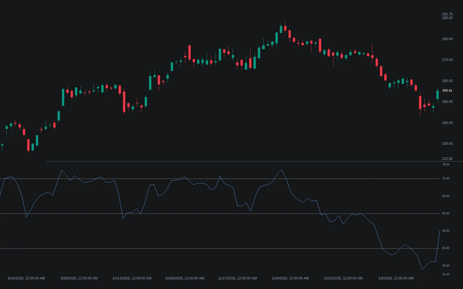
The Python engine is the right tool when you need full control: custom data, portfolio-level tests, unusual fill models. For the common case, testing a rule against a chart's data with realistic costs, the work is already done. Describe the rule to Quant in plain language, for example a long when the 14-period RSI closes below 30, flat when it closes above 70, with a 2% stop. Quant writes the strategy in Pine Script, the industry's chart scripting language, and plots it on the active chart. Open Code to read the script and confirm the entries are evaluated on closed bars, then click Run. The Making Strategies with Quant guide covers the workflow, including converting an existing indicator into a strategy with the Backtest button.
Reading the Backtest
A Backtest Summary strip appears below the chart with net profit, trade count, win rate, maximum drawdown and profit factor, and the full viewer adds a Performance tab with the equity curve and a long-versus-short split, a Trades Analysis tab with the P&L distribution and duration views, and a searchable Trades Log. The native backtest guide explains each. Two properties deserve attention before any number is trusted: commission and slippage default to zero and must be set realistically, and the symbol and timeframe can be changed inside the viewer to re-run the same strategy on different data, which is the quickest out-of-sample check available. Starred runs save the script, symbol, timeframe, inputs and properties together, so every result stays reproducible.
| Question | Python engine | Quant on Quant Charts |
|---|---|---|
| Who writes the code? | You, in Python | Quant, in Pine Script, from your description; editable in Code |
| Where does the data come from? | Files or APIs you manage | The chart's own feed for the active symbol and timeframe |
| Costs and fills | Whatever you model, and whatever you forget | Commission, slippage, order size, pyramiding and margin in Properties |
| Reporting | Whatever you compute | Summary strip plus Performance, Trades Analysis and Trades Log tabs |
| Portfolio and multi-asset tests | Yes, with more code | One symbol per run; switch symbols inside the viewer |
| Live orders | Only if you build the broker connection yourself | The LuxAlgo platform does not place orders for you |
Conclusion
A backtesting engine is a machine for making assumptions explicit. The data module decides what the strategy is allowed to know, the signal layer decides when it is allowed to know it, the execution loop decides what a trade costs, and the metrics decide what counts as success. Build each part small, test it against cases you can check by hand, and charge costs from the first run. Then validate out of sample, because an in-sample result is a hypothesis and nothing more. When the question is simply whether a rule works on a chart with realistic costs, Quant can write and run it for you; when the question needs custom data or a portfolio view, the Python engine is worth the afternoon it takes to build.
Key Takeaways
- Four modules, narrow interfaces. Data, signals, execution and metrics should each be replaceable without touching the others.
- Shift signals, fill at the next open. That one convention removes most look-ahead bias.
- Costs are part of the strategy. A $7.50 round trip turned a 1.83 profit factor into 1.65 in the worked example; set them before you read any result.
- Validate, then validate again. Holdout, walk-forward and robustness tests separate an edge from a curve fit.
- Quant does the common case. Describe a rule, inspect the Pine Script in Code, click Run, and read the Backtest Summary with commission and slippage set.
FAQs
What is the difference between event-driven and vectorised backtesting?
A vectorised backtest computes signals and returns for the whole series at once with array operations; it is fast but makes it easy to fill at prices that were not yet known. An event-driven engine walks bars in order, deciding on one bar and filling on the next, so costs, fills and risk rules can be applied per trade. Use vectorised code for quick screening and an event loop for anything you might trade.
How do I avoid look-ahead bias in a Python backtest?
Compute every indicator from data up to the current bar, shift the resulting signal forward by one bar, and fill at the next bar's open rather than the signal bar's close. Test the engine on a toy series where you know the correct trades. Be equally careful with adjusted data and with any field, such as a daily high, that is only known once the bar has closed.
Which metrics should a backtesting engine report?
Net profit and total return, maximum drawdown, trade count, win rate with average win and loss, profit factor, expectancy per trade, Sharpe or Sortino ratio, and exposure and turnover. Read the drawdown and the trade count before the return, and never read the win rate without the average win and loss beside it.
How much should I charge for commission and slippage?
Enough that the backtest is pessimistic. A few basis points per side for liquid stocks and major crypto pairs is a common starting point, more for thin names, and gaps through stops should fill at the open rather than at the stop price. In the worked example a $7.50 round trip removed a fifth of the rule's edge; leaving costs at zero flatters every strategy.
How do I know if a backtest is overfitted?
Hold out data before you look at any result and read it once; run walk-forward analysis to see whether re-optimised parameters wander; check that neighbouring parameter values give similar results; remove the best few trades and see whether the edge survives. A result that only exists at one exact setting on one exact sample is a curve fit.
Can I backtest without writing Python?
Yes. Describe the rule to Quant on Quant Charts, including entries, exits and risk rules; Quant writes the strategy in Pine Script, which you can inspect in Code, and Run produces a Backtest Summary with net profit, trade count, win rate, maximum drawdown and profit factor. Set commission and slippage in Properties, and re-run on other symbols and timeframes from the viewer as an out-of-sample check.
References
LuxAlgo Resources
- Quant Charts
- LuxAlgo Quant
- What Is Quant?
- Making Strategies with Quant
- Native Backtest Guide
- Relative Strength Index Indicator
- RSI
- Expectancy
- Drawdown Statistics
- Sharpe Ratio
- Sortino Ratio
- Execution Cost Modeling
- In-Sample / Out-of-Sample Split
- Walk-Forward Analysis
- Parameter Stability
- Robustness Testing
- Stress-Test Your Algorithmic Trading Strategy
- In-Sample Testing vs Out-of-Sample Testing
- Backtesting Limitations: Slippage and Liquidity Explained
- Walk-Forward Testing vs Backtesting
- Backtesting vs Forward Testing
- Building Your First Trading Bot
External Resources
Read next