Deep Learning Applications in Algorithmic Trading
Deep learning in algorithmic trading means fitting multi-layer neural networks to market data so they learn the mapping from inputs to a forecast or a decision, instead of a trader writing the rule by hand. The architectures are well understood: feed-forward networks for tabular features, recurrent networks such as the LSTM for sequences, convolutional networks for local patterns, transformers for text and long contexts, and reinforcement learning when the output is an action rather than a prediction. What is less understood is how rarely these models beat simple baselines once they are evaluated honestly, with time-ordered splits and trading costs. This guide covers the architectures and what each is suited to, what the published research actually shows, the pipeline discipline that separates a real result from a curve fit, the pitfalls specific to financial data, and where LuxAlgo fits: the Library's machine-learning family of transparent on-chart tools, and Quant, our coding agent, which writes the deterministic rule a trained model produces as Pine Script on Quant Charts and backtests it with costs.
Key points:
- Architecture matters less than labels, features and validation. What you ask the network to predict, over what horizon, tested on data it never saw, decides whether the result means anything.
- Returns are hard; volatility is easier. Sequence models earn their keep on persistent quantities and on text, not on next-bar direction of liquid markets.
- Time-ordered validation is non-negotiable. Random shuffles, scaling fitted on the whole sample and overlapping labels all leak the future into training.
- A chart cannot train an LSTM. Training happens offline; the chart is where the resulting rule is expressed, tested and monitored.
Which Architecture Fits Which Problem
| Architecture | What it models | Typical trading inputs | Honest caveat |
|---|---|---|---|
| Feed-forward network (MLP) | A flexible function of fixed-length features | Engineered features: returns, volatility, indicator values, fundamentals | Often no better than gradient-boosted trees on the same tabular features, and harder to tune |
| Recurrent network (LSTM, GRU) | Sequences with a carried hidden state; LSTM gates learn what to remember | Windows of returns and features; volatility series | Regularly fails to beat simpler baselines on liquid-market returns out of sample; stronger on volatility |
| Convolutional network (CNN) | Local patterns across a window or an image | Multichannel price and indicator windows; order-book snapshots; chart images | Chart-image approaches throw away numeric precision the network then has to relearn |
| Transformer | Attention over long contexts; the architecture behind large language models | News, filings and transcripts; long multivariate sequences | Text signals decay quickly and are crowded; needs a lot of data for numeric series |
| Deep reinforcement learning | A policy that maps state to action to maximise reward | Portfolio weights, order placement, execution scheduling | Reward design and simulator realism dominate results; sample-inefficient and fragile across regimes |
The Library's neural networks and LSTM and recurrent networks entries give the technical background. The LSTM was introduced by Hochreiter and Schmidhuber in 1997 to fix the vanishing-gradient problem that made plain recurrent networks forget long-range context; the transformer, introduced by Vaswani and colleagues in 2017, replaced recurrence with attention and has since displaced recurrent models across most of the research literature.
What the Research Shows
Three findings are worth carrying into any project. First, a systematic review of financial time-series forecasting studies from 2005 to 2019 by Sezer, Gudelek and Ozbayoglu found deep learning models reporting results that significantly outperform traditional machine-learning counterparts across the literature; the same review is a catalogue of how varied and hard to compare those studies are, with different assets, horizons, metrics and, usually, no trading costs. Second, Gu, Kelly and Xiu's work on empirical asset pricing via machine learning showed that flexible methods, trees and neural networks in particular, improve out-of-sample return prediction over linear models on a broad cross-section of US stocks, with the gains concentrated in nonlinear interactions among a handful of known predictors. Third, deep reinforcement learning has been shown to learn an adaptive allocation over a basket of large stocks and to compare favourably with the index and a minimum-variance portfolio in the authors' test, as in Xiong and colleagues' 2018 paper, while depending heavily on the realism of the training environment.
The honest summary is the one the Library's LSTM entry gives: on liquid markets, sequence models regularly fail to beat much simpler baselines once evaluated strictly out of sample with costs. The published accuracy figures that circulate in marketing, often above 90 percent, come from in-sample fits, from predicting levels rather than returns, or from short windows, and should be treated as red flags rather than benchmarks.
Where Deep Learning Is Used
- Direction and return prediction. The classic target and the hardest. Results improve when the label is a risk-adjusted or volatility-scaled return over a defined horizon rather than a raw next-bar sign, and when the feature set is small and economically motivated.
- Volatility forecasting. Volatility clusters and persists, which is exactly what a recurrent network captures. Forecasting realised volatility to size positions or price options is where LSTMs and GRUs have the strongest case.
- Text and sentiment. Transformers turn news, filings and transcripts into features: event detection, tone, topic exposure. The Library's LLM and transformer-derived signals entry covers the approach and its limits; the information is real, fleeting and crowded.
- Allocation and execution. Reinforcement learning frames rebalancing or order scheduling as sequential decisions. Our guides to reinforcement learning for portfolio rebalancing and reinforcement learning in market simulations go deeper; the Library's reinforcement-learning policies entry explains why the simulator matters more than the algorithm.
- Regime detection. Unsupervised or lightly supervised models that classify the market state, so a rule-based system can switch parameters or stand aside. Often the highest-value and lowest-risk use, because the model gates a strategy rather than trading on its own.
Building the Pipeline
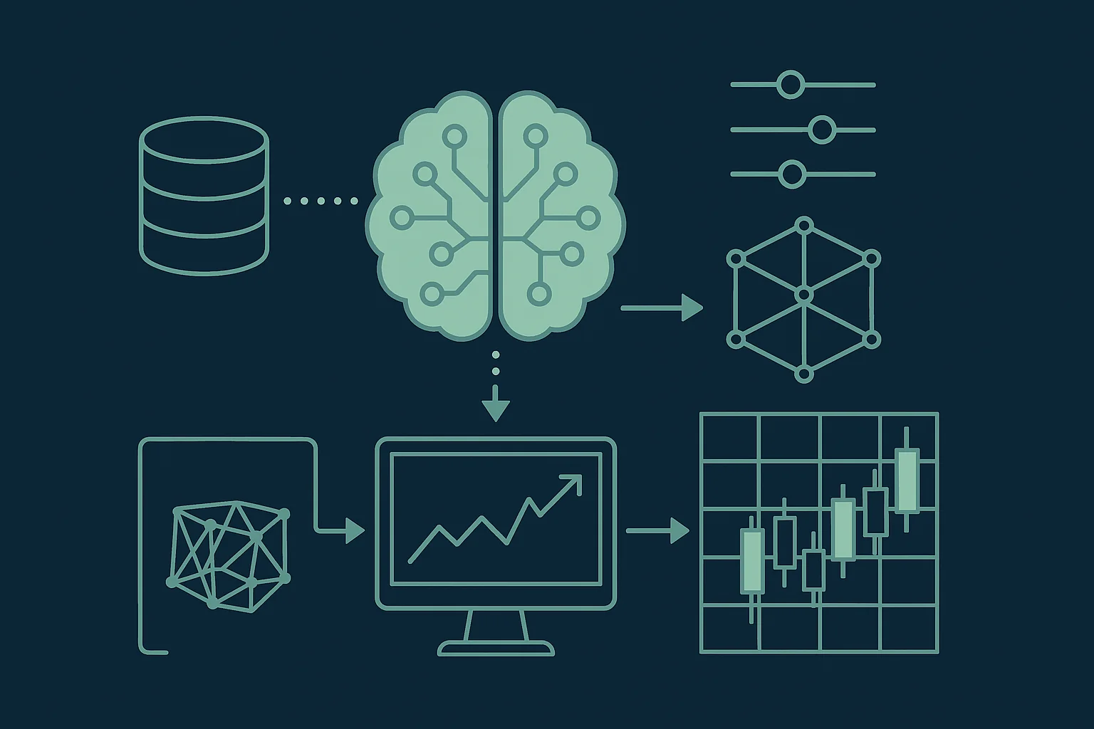
The Library's feature engineering and in-sample and out-of-sample split entries describe the two ends of this pipeline; the steps between them are where most projects fail.
- Define the label and horizon first. Next-bar sign, five-day volatility-scaled return, realised volatility over twenty bars: each is a different problem with different noise. Overlapping labels, where consecutive samples share future bars, are the first source of leakage.
- Engineer a small feature set from returns, ranges, volume and a few indicators, each stationary or made stationary by differencing or normalisation. Raw prices from different years are not comparable inputs.
- Split by time, never at random. Train on the past, validate on the next block, test on the block after that. Purge samples whose labels overlap the split boundary and leave an embargo gap so no information crosses.
- Fit scalers and any encoders on the training block only, then apply them forward. Fitting on the full sample is the second, quieter source of leakage.
- Walk forward. Retrain on an expanding or rolling window and evaluate each subsequent block, so the reported result is an average over many out-of-sample periods rather than one lucky split. Our guide to walk-forward testing versus backtesting covers the mechanics.
- Convert predictions into positions and charge costs. A classifier's accuracy is not a trading result; a backtest with commission and slippage over the walk-forward predictions is.
- Plan retraining and monitoring before deployment, since a model fitted to one regime degrades in the next.
A Minimal Time-Ordered Training Loop
The snippet trains a small LSTM classifier in PyTorch on windows of standardised returns, using scikit-learn's time-series splitter so that every validation block lies after its training block and the scaler is fitted only on training data. It is a skeleton to build on, not a strategy.
import numpy as np
import torch
import torch.nn as nn
from sklearn.model_selection import TimeSeriesSplit

# returns: 1-D numpy array of daily log returns, oldest first
WINDOW, HORIZON = 20, 5

def make_samples(r):
    X, y = [], []
    for i in range(WINDOW, len(r) - HORIZON):
        X.append(r[i - WINDOW:i])
        y.append(1.0 if r[i:i + HORIZON].sum() > 0 else 0.0)   # label: sign of the forward 5-day return
    return np.array(X), np.array(y)

X, y = make_samples(returns)

class LSTMClassifier(nn.Module):
    def __init__(self, hidden=16):
        super().__init__()
        self.lstm = nn.LSTM(input_size=1, hidden_size=hidden, batch_first=True)
        self.head = nn.Linear(hidden, 1)
    def forward(self, x):
        out, _ = self.lstm(x.unsqueeze(-1))
        return self.head(out[:, -1, :]).squeeze(-1)

scores = []
for train_idx, test_idx in TimeSeriesSplit(n_splits=5, gap=HORIZON).split(X):
    # scaler statistics from the training block only; the gap purges overlapping labels
    mu, sd = X[train_idx].mean(), X[train_idx].std() + 1e-9
    Xtr = torch.tensor((X[train_idx] - mu) / sd, dtype=torch.float32)
    Xte = torch.tensor((X[test_idx] - mu) / sd, dtype=torch.float32)
    ytr = torch.tensor(y[train_idx], dtype=torch.float32)

    model = LSTMClassifier()
    opt = torch.optim.Adam(model.parameters(), lr=1e-3)
    loss_fn = nn.BCEWithLogitsLoss()
    for epoch in range(20):
        opt.zero_grad()
        loss = loss_fn(model(Xtr), ytr)
        loss.backward()
        opt.step()

    with torch.no_grad():
        pred = (torch.sigmoid(model(Xte)) > 0.5).float().numpy()
    scores.append((pred == y[test_idx]).mean())

print("out-of-sample accuracy per block:", np.round(scores, 3))
print("baseline (always up):", np.round(y.mean(), 3))
Two habits in the snippet matter more than the network. The splitter's gap purges samples whose five-day labels would straddle the boundary, and the mean and standard deviation come from the training block alone. Compare each block's accuracy with the always-up baseline printed at the end; a model that cannot beat it consistently has learned nothing tradable, however elaborate its architecture.
Pitfalls Specific to Financial Data
| Pitfall | How it shows up | Defence |
|---|---|---|
| Look-ahead leakage | Scalers, features or labels use information from after the prediction time | Fit everything on the training block; as-of alignment; purge and embargo around splits |
| Random shuffling | Adjacent, nearly identical windows land in both train and test | Time-ordered splits only; walk-forward evaluation |
| Overlapping labels | Consecutive samples share future bars, inflating apparent sample size | Gap equal to the horizon between train and test; weight or thin overlapping samples |
| Non-stationarity | A model fitted to one regime fails in the next | Stationary features; rolling retraining; regime gating |
| Low signal-to-noise | Networks memorise noise; training loss falls while test loss does not | Small models, strong regularisation, early stopping, fewer features |
| Multiple testing | Dozens of architectures tried, the best reported | Hold out a final test block touched once; report all attempts |
| Costs ignored | Accuracy reported, returns after costs never computed | Backtest predictions as positions with commission and slippage |
| Opaque failure | The model stops working and nobody can say why | Monitoring, drift detection, and a documented retraining and shutdown policy |
The Regulatory Direction
Regulators have started to ask how these systems are governed. In January 2024 the Commodity Futures Trading Commission's staff issued a request for comment on the current and potential uses and risks of artificial intelligence in the derivatives markets it regulates, to inform whether future guidance or rules are needed. The practical implication for anyone deploying a model is unchanged by jurisdiction: document the data, the training, the validation and the monitoring, and be able to explain what the system does and how it is switched off.
Where LuxAlgo Fits
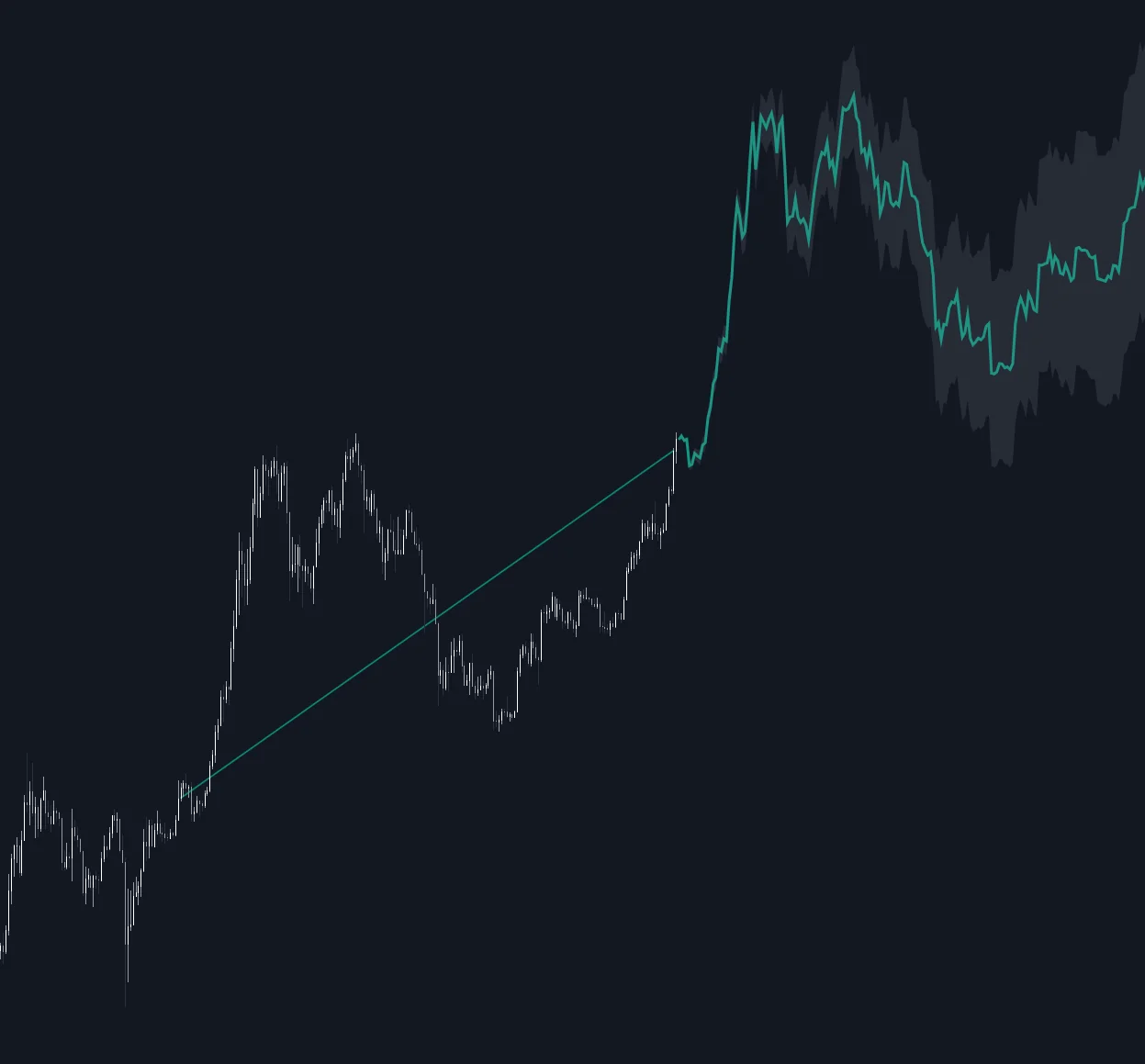
The Library's machine-learning family is deliberately built from methods that fit on the fly to visible history and can be inspected: kNN analog forecasting, implemented by The Echo Forecast and Historical Price Projection, kernel regression, clustering for regime detection and gradient boosting. Its LSTM entry explains why there is no on-chart deep network: an LSTM is a trained artifact that needs a labelled dataset, time-ordered splits, scaling fitted on past data and scheduled retraining, none of which a chart script can provide, and scripts marketed as on-chart LSTMs are either frozen stale weights or in-sample curve fits.
The workflow that does work is to train offline and express the result on the chart. A trained model usually reduces to something deterministic at the point of use: a threshold on a feature, a regime label that gates entries, a volatility forecast that sizes positions. Describe that rule to Quant, go long only when twenty-day realised volatility is below its rolling median and the fast average has crossed the slow, and Quant writes it in Pine Script on the active Quant Charts symbol. Open Code to read the logic, click Run, and the Backtest Summary reports net profit, trade count, win rate, maximum drawdown and profit factor, with commission and slippage set in the strategy properties, so the walk-forward result from the training pipeline is checked against a cost-aware backtest on the chart. The Making Strategies with Quant guide shows the steps, and PineTS, LuxAlgo's TypeScript implementation of Pine Script, lets the same indicator and strategy logic run inside a TypeScript pipeline alongside a Python or JavaScript model.
Two boundaries. The LuxAlgo platform does not place orders for you; Quant Charts is where rules are written and tested, and execution stays with your broker or your own code, for example through our open-source Trade Relay and Broker SDK. And a backtest is a simulation under the costs you set, not a forecast. For the surrounding engineering, see our guides to Python libraries for algorithmic trading, building a backtesting engine in Python and ensemble learning for chart patterns.
Conclusion
Deep learning gives traders a set of flexible function approximators, and the research shows they can add predictive value, most clearly on volatility, on text and in nonlinear interactions among known predictors. It also shows how easily the results are faked by leakage, shuffling, overlapping labels and ignored costs. The pipeline discipline in this guide, labels first, stationary features, time-ordered splits with purging, scalers fitted on training data, walk-forward evaluation and a cost-aware backtest, is what separates a model from a curve fit. When the model produces a rule, Quant writes it in Pine Script on Quant Charts and the Backtest Summary judges it with costs, which is where every model should have to prove itself before it trades.
Key Takeaways
- Match the architecture to the problem. MLPs for features, recurrent networks for persistent sequences like volatility, transformers for text, reinforcement learning for decisions.
- Distrust high accuracy. Published figures above 90 percent almost always mean leakage, level prediction or a short window.
- Validate in time order with purging, an embargo and scalers fitted on the training block only.
- Charge costs and compare with a baseline before calling anything a result.
- Train offline, express on the chart. Quant writes the resulting rule in Pine Script; the Backtest Summary reports the outcome; no LuxAlgo tool places orders.
FAQs
What is deep learning in algorithmic trading?
Using multi-layer neural networks, trained on historical market and alternative data, to learn a forecast or a decision rule instead of specifying it by hand. Common targets are the direction or size of future returns, future volatility, text-derived sentiment, market regime, and portfolio or execution decisions learned through reinforcement learning.
Which neural network is best for stock prediction?
None is best in general. Feed-forward networks suit engineered tabular features and are often matched by gradient-boosted trees; LSTMs and GRUs suit persistent sequences such as volatility; transformers suit text and long contexts; reinforcement learning suits decisions. The label, the features and the validation scheme usually matter more than the architecture.
How accurate are LSTM stock predictions?
Evaluated honestly, with time-ordered splits, purged overlapping labels and trading costs, LSTMs on liquid-market returns regularly fail to beat simple baselines. Figures above 90 percent that circulate online usually come from in-sample fits, from predicting price levels rather than returns, or from short windows. Volatility forecasting is where recurrent networks have the strongest record.
How do I avoid overfitting a trading model?
Split data by time rather than at random, leave a gap equal to the label horizon between training and test blocks, fit scalers only on training data, keep the model and feature set small, use early stopping and regularisation, hold out a final test block that is touched once, and evaluate with walk-forward retraining and a cost-aware backtest rather than a single accuracy number.
Can I run a deep learning model on a chart?
Not as a training process. A chart script sees one symbol's loaded history and has no dataset, no time-ordered training pipeline and no retraining schedule, so on-chart LSTMs are either frozen stale weights or in-sample curve fits. Train offline, then express the model's output as a deterministic rule on the chart. The Library's machine-learning family offers transparent alternatives such as kNN analog forecasting and kernel regression.
How does Quant help with deep learning strategies?
Quant, LuxAlgo's coding agent, writes the deterministic rule a trained model produces, a threshold, a regime gate or a volatility-based size, as Pine Script on Quant Charts. Open Code to read it, click Run, and the Backtest Summary reports net profit, trade count, win rate, maximum drawdown and profit factor with commission and slippage in the strategy properties. PineTS lets the same logic run in TypeScript pipelines. No LuxAlgo tool places orders.
References
LuxAlgo Resources
- Quant Charts
- LuxAlgo Quant
- Making Strategies with Quant
- PineTS Documentation
- Library: Machine Learning Family
- Neural Networks Concept
- LSTM and Recurrent Networks Concept
- Feature Engineering Concept
- In-Sample and Out-of-Sample Split Concept
- kNN Analog Forecasting Concept
- Kernel Regression Concept
- Reinforcement-Learning Policies Concept
- LLM and Transformer-Derived Signals Concept
- The Echo Forecast Indicator
- Historical Price Projection Indicator
- Walk-Forward Testing vs Backtesting
- Reinforcement Learning for Portfolio Rebalancing
- Reinforcement Learning in Market Simulations
- Ensemble Learning for Chart Patterns
- How to Build a Backtesting Engine in Python
- Python for Algorithmic Trading: Essential Libraries
- Backtesting Traps: Common Errors to Avoid
External Resources
- Wikipedia — Long Short-Term Memory
- Vaswani et al. — Attention Is All You Need (arXiv, 2017)
- Sezer, Gudelek and Ozbayoglu — Financial Time Series Forecasting with Deep Learning: A Systematic Literature Review 2005–2019 (arXiv)
- Gu, Kelly and Xiu — Empirical Asset Pricing via Machine Learning (NBER)
- Xiong et al. — Practical Deep Reinforcement Learning Approach for Stock Trading (arXiv, 2018)
- scikit-learn — Cross-Validation and TimeSeriesSplit
- Wikipedia — Leakage (Machine Learning)
- Wikipedia — Overfitting
- CFTC — Staff Request for Comment on the Use of Artificial Intelligence in CFTC-Regulated Markets (January 2024)
- PyTorch
- TensorFlow
Read next