Machine Learning in Risk Parity Analysis

Risk parity is an allocation rule: instead of dividing capital equally or by expected return, it divides risk equally, so that each holding contributes a similar share of the portfolio's volatility. The idea is older than the machine-learning vocabulary now attached to it, and most of what machine learning changes is upstream of the rule itself, in how volatilities, correlations and regimes are estimated before the weights are computed. This guide explains, from the LuxAlgo Library's documentation, Bridgewater's account of the strategy's origin and the SEC's investor guidance, what risk parity actually computes, where its inputs come from, what clustering, regime models and learned forecasts add and what they cost in validation, and how the watchlist, Journal and Quant tools in Quant Charts support the parts of this work an individual trader can do. It replaces the accuracy percentages that circulate in this topic with what the sources support.
What Risk Parity Computes
The Library's Portfolio-aware Sizing entry files risk parity under sizing schemes that set each position with reference to everything else the account holds. Its definition is direct: allocate so each position contributes a similar share of portfolio volatility, extending volatility-targeted sizing to the book level. Portfolio volatility is the square root of the sum over every pair of positions of the two weights, the two volatilities and their correlation, so two holdings that move together behave as one larger position. The closed-form shortcut is inverse-volatility weighting, where each weight is the reciprocal of the asset's volatility divided by the sum of those reciprocals; the Library notes this matches full risk parity exactly when all pairwise correlations are equal, and that the full version, which equalises each position's contribution to portfolio volatility, needs a numeric solver.
The strategy's institutional origin is documented by Bridgewater in The All Weather Story, which describes the All Weather portfolio launched in 1996 as the foundation of the risk parity movement. The premise was that asset classes react in understandable ways depending on how their cash flows relate to the economic environment, so a portfolio could be balanced by those structural characteristics rather than by predicting which environment comes next. The account describes a four-box diagram of rising and falling growth and inflation, with the key being to put equal risk on each scenario, and it records that a little leverage had to be applied to inflation-linked bonds to bring their risk up to the rest. The SEC's investor guidance makes the same underlying point in plainer language: including asset categories whose returns move up and down under different conditions protects against significant losses, because historically the major categories have not moved together.
Where the Inputs Come From
Every risk parity weight is only as good as the volatility and correlation estimates behind it, and all of those look backward. The Library's Volatility-targeted Sizing entry states the problem: when volatility jumps faster than the lookback updates, through news, gaps or a regime break, the position sized for yesterday's range takes today's larger one, and the realised loss can exceed the budget. Volatility targeting standardises an estimate of risk; it does not cap the outcome.
- Volatility. Realized volatility measures what an asset actually printed over a window, and EWMA volatility weights recent squared returns more heavily with a decay factor, 0.94 for daily data in the RiskMetrics convention, so turbulent periods are recognised sooner without any model fitting.
- Correlation. The Library's Correlation entry insists on computing it on returns over a rolling window, because raw trending prices produce inflated, spurious readings, and traces the covariance matrix's central role to Markowitz's 1952 portfolio theory, whose assumptions every risk model since has inherited.
- Sizing base. The parity weights feed the portfolio volatility check, and the Library layers further controls on top: a total open-risk ceiling, commonly around 6 percent of equity, and a capped Kelly fraction, with the reminder that Kelly assumes independent bets so correlated positions argue for a smaller multiplier.
What Machine Learning Changes
Machine learning enters risk parity at three points, and the Library documents each method with its limits.
Regime detection. A single volatility estimate assumes one market state. K-means regime clustering partitions recent feature values, such as ATR readings, realised volatility or trend-strength measures, into data-defined low, medium and high states, so that what counts as quiet or volatile is decided by recent data rather than fixed thresholds; its classical limits are that the number of clusters is chosen in advance, convergence is to a local optimum, and the clusters describe the present without forecasting the next state. Hidden Markov and Markov-switching models go further, describing the market as moving between unobserved states with a transition matrix whose fitted self-transition probabilities are typically high, so regimes tend to persist; the states carry no built-in meaning, and labels such as bull or bear are assigned by inspecting the fitted parameters afterwards. Either approach lets a risk parity book use regime-conditional volatilities and correlations instead of one unconditional estimate.
Hierarchical clustering and Hierarchical Risk Parity. Marcos López de Prado's 2016 paper in the Journal of Portfolio Management introduced Hierarchical Risk Parity as an alternative to inverting a covariance matrix that is estimated with error. The method converts the correlation matrix into distances, builds a tree by hierarchical clustering so that similar assets are grouped, reorders the covariance matrix so that similar assets sit together, and then splits the risk budget recursively down the tree, allocating between the two halves of each split in inverse proportion to their variance. Because it never inverts the covariance matrix, it avoids the instability that makes mean-variance weights swing wildly when inputs change slightly, and its stated aim is portfolios that hold up out of sample. Whether it does so for a given universe and period is an empirical question for the validation methods below, not a settled fact.
Learned forecasts. The volatility and correlation inputs can themselves be predicted by supervised models. The Library describes random forests, ensembles of decision trees whose errors partially cancel and which ship with out-of-bag error and feature importance diagnostics; support vector machines, maximum-margin classifiers that remain a common baseline for scarce data; and neural networks, function approximators whose flexibility is both the appeal and the hazard, since a network with enough parameters can memorise noise and in-sample accuracy means little. Reinforcement learning frames sizing itself as the decision to be learned; the Library's summary of the field's experience is that the framework fits the problem beautifully and the data fights it viciously. Every one of these models runs on engineered features that must be roughly stationary and computable strictly from data available at prediction time, and PCA is the standard way to compress a large correlated feature set before a model sees it.
| Allocation method | Inputs | What it equalises | Main weakness |
|---|---|---|---|
| Equal weight | None | Capital | Risk concentrates in the most volatile holdings |
| Inverse volatility | Volatility per asset | Standalone volatility contribution | Ignores correlations; matches parity only when correlations are equal |
| Full risk parity | Volatilities and correlations | Contribution to portfolio volatility | Needs a solver; estimates look backward |
| Hierarchical Risk Parity | Correlation distances, variances | Risk within a clustered tree | Depends on the clustering and linkage choices |
| Regime-conditional parity | Any of the above, per detected regime | Risk within the current state | Regime detection lags and can misclassify |
The Validation Burden
Adding learned components to an allocation rule multiplies the ways a backtest can flatter it, and the Library's validation entries are the answer. An in-sample and out-of-sample split holds back a later block until the design is frozen, because parameters tuned on one stretch always look good on that stretch. Walk-forward analysis repeats the split, re-optimising on each window and applying the result to the next unseen one, which is a rehearsal of exactly the periodic re-estimation a risk parity book performs. The probability of backtest overfitting evaluates the research process rather than one configuration, asking how often the in-sample winner among all the variants tried lands in the bottom half out of sample. Investor.gov's guidance on rebalancing fits the same discipline: rebalance on a calendar or when an allocation drifts past a threshold set in advance, and expect rebalancing to work best when done relatively infrequently, which argues against models that reallocate on every new estimate.
Limitations
- Backward-looking inputs. Every estimate is of the past, and the Library's sizing entries are explicit that a volatility jump can push the realised loss past the budget before the estimate catches up.
- Correlations that converge in stress. Diversification measured in calm periods can vanish when assets fall together, which is the scenario the four-box balancing was designed for and the one a learned correlation forecast most needs to get right.
- Leverage. Equalising risk across assets with very different volatilities generally requires levering the low-volatility ones, as Bridgewater's account of inflation-linked bonds shows; that introduces financing and liquidity risk the weights do not display.
- Overfitting. Regime models, clusterings and forecasters each add parameters; the Library treats an out-of-sample or walk-forward test as non-negotiable for any learned component.
- Unverifiable claims. Accuracy percentages for machine-learning risk models circulate widely without reproducible sources. None are quoted here, and none should be relied on without the underlying data and method.
Where Quant Charts Fits
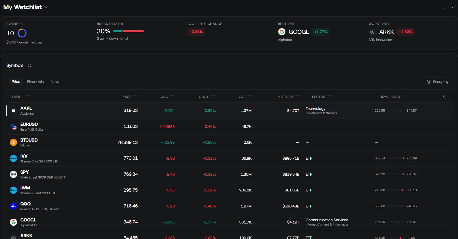
See the book's exposure. Build a watchlist of your holdings and open the Advanced view. Its Allocation section shows an asset-class donut across stocks, ETFs, crypto, forex and commodities with a 24-hour change breakdown, and a sector exposure view for stocks and ETFs, so concentration by class and sector is visible before any weight is computed. Sections let you group holdings into the sleeves you intend to balance, and the Financials tab reports beta for stocks as a first read on how a name moves with the market.
The video below shows how favourites and the indicator wheel work in Quant Charts.
Measure the inputs on the chart. The LuxAlgo Library is built into the Indicators picker, and its statistics and volatility families include rolling correlation, realised and EWMA volatility and k-means regime clustering indicators that plot the quantities a parity rule consumes. Reading a rolling correlation between two holdings on returns, as the Library specifies, is the fastest way to see how much of your diversification is real.
Test a volatility-scaled rule. Describe a per-symbol rule to Quant, our coding agent, in plain language: for example, size each entry so that one ATR multiple of adverse movement equals a fixed fraction of equity, and reduce size when the k-means regime is high volatility. Quant writes the Pine Script; open Code to inspect it, then click Run. The Backtest Summary reports net profit, trade count, win rate, max drawdown and profit factor, with commission and slippage set in the strategy's Properties. Re-run the same strategy on other symbols from inside the viewer and sweep the volatility lookback to check that the result does not hinge on one setting.
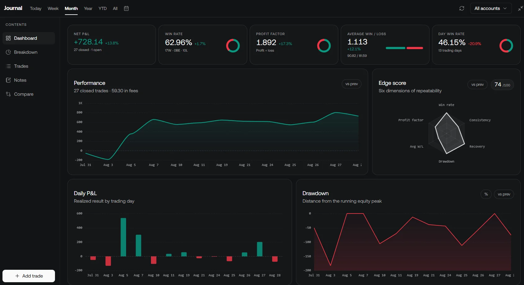
Journal the realised risk. Every plan includes the Journal, which turns broker fills or imported trades into round trips and reports win rate, profit factor and drawdown with a breakdown by hold time, day, time of day, symbol and side. The breakdown by symbol is the realised version of a risk budget: if one holding accounts for most of the drawdown, the book was not at parity whatever the weights said.
What the platform does not do. Quant Charts does not run portfolio optimisation, compute covariance matrices across a book or implement Hierarchical Risk Parity, and no LuxAlgo tool places orders. It charts the inputs, tests single-symbol rules and records the outcomes; the allocation model itself lives in your own tooling.
FAQs
What is risk parity?
An allocation rule that sizes each holding so it contributes a similar share of portfolio volatility, rather than an equal share of capital. The inverse-volatility shortcut divides each asset's reciprocal volatility by the sum of all reciprocals and matches full parity when correlations are equal; full parity needs a solver.
Where did risk parity come from?
Bridgewater's All Weather Story describes the All Weather portfolio, launched in 1996, as the foundation of the risk parity movement: assets balanced by how their cash flows respond to growth and inflation, with equal risk placed on each of four economic scenarios and leverage applied to low-volatility assets such as inflation-linked bonds.
What is Hierarchical Risk Parity?
A method introduced by Marcos López de Prado in 2016 that clusters assets by correlation distance into a tree, reorders the covariance matrix so similar assets sit together, and splits the risk budget recursively down the tree in inverse proportion to variance, avoiding the matrix inversion that makes mean-variance weights unstable.
What does machine learning add to risk parity?
Regime detection with k-means or Markov-switching models so volatilities and correlations are conditional on the current state, hierarchical clustering of the asset universe, and learned forecasts of the inputs with random forests, support vector machines or neural networks. Each adds parameters and therefore validation burden.
What are the main risks of a machine-learning risk parity model?
Backward-looking inputs that lag volatility jumps, correlations that converge in stress, leverage on low-volatility assets, overfitting of regime models and forecasters, and reliance on accuracy claims that cannot be reproduced. Out-of-sample and walk-forward testing are the minimum defences.
Can Quant Charts run a risk parity portfolio?
No. It shows allocation and sector exposure in the watchlist Advanced view, plots correlation, volatility and regime indicators from the Library, lets Quant test volatility-scaled sizing rules per symbol, and records realised risk by symbol in the Journal. Portfolio optimisation and order placement happen outside the platform.
References
LuxAlgo Resources
- Portfolio-aware Sizing, Volatility-targeted Sizing, Correlation, Realized Volatility and EWMA Volatility concepts (LuxAlgo Library)
- K-means Regime Clustering, Hidden Markov / Markov-switching Regimes, Random Forest, Support Vector Machines, Neural Networks, Reinforcement-learning Policies, Feature Engineering and PCA concepts (LuxAlgo Library)
- In-sample / Out-of-sample Split, Walk-forward Analysis and Probability of Backtest Overfitting concepts (LuxAlgo Library)
- Watchlist Advanced view, Journal Breakdown, Making strategies with Quant and Strategies and the Backtest viewer (LuxAlgo Docs)
External Resources
- The All Weather Story, January 2012 (Bridgewater Associates)
- Beginners' Guide to Asset Allocation, Diversification, and Rebalancing (Investor.gov, U.S. Securities and Exchange Commission)
- Marcos López de Prado, Building Diversified Portfolios that Outperform Out of Sample, Journal of Portfolio Management, 2016 (the source of Hierarchical Risk Parity; described above from the published method)
This article is educational and is not investment advice. Risk parity and machine-learning allocation models depend on estimates of volatility and correlation that can fail in stress, and no allocation method guarantees a return or limits a loss.
Read next