How to Adjust Moving Averages for Volatile Markets
Adjusting a moving average means choosing how much responsiveness to exchange for smoothing. A shorter lookback or larger smoothing coefficient responds more quickly, but can also react more often to movements that reverse. High volatility does not automatically call for a faster average: a volatile trend and a volatile sideways market pose different problems.
Start with the exact formula, chart interval and decision rule. Compare a small set of settings under realistic costs, then evaluate them on data excluded from selection. Adaptive averages can change their responsiveness according to a specified input; they do not automatically produce more accurate or profitable signals.
Choose the Formula Before Changing the Settings
| Average | What controls its response | Important limitation |
|---|---|---|
| Simple moving average (SMA) | An equally weighted window of observations | Changing the window trades responsiveness against smoothing |
| Exponential moving average (EMA) | A fixed recursive smoothing coefficient for the selected length | Recent prices receive more weight, but turning points are still uncertain |
| Variable moving average (VMA) | An implementation-specific changing coefficient or period | The name alone does not identify the adaptation rule |
| CMO-based VIDYA | An EMA coefficient multiplied by normalized absolute momentum imbalance | Large alternating moves can produce low responsiveness despite high volatility |
“Variable moving average” is a broad label. Check the documentation or code rather than assuming that every VMA uses the same input. VIDYA implementations also need to be identified explicitly. The MetaQuotes VIDYA reference documents a version based on the Chande Momentum Oscillator (CMO), so VIDYA should not be described universally as a standard-deviation average.
Understand What CMO-Based Adaptation Measures
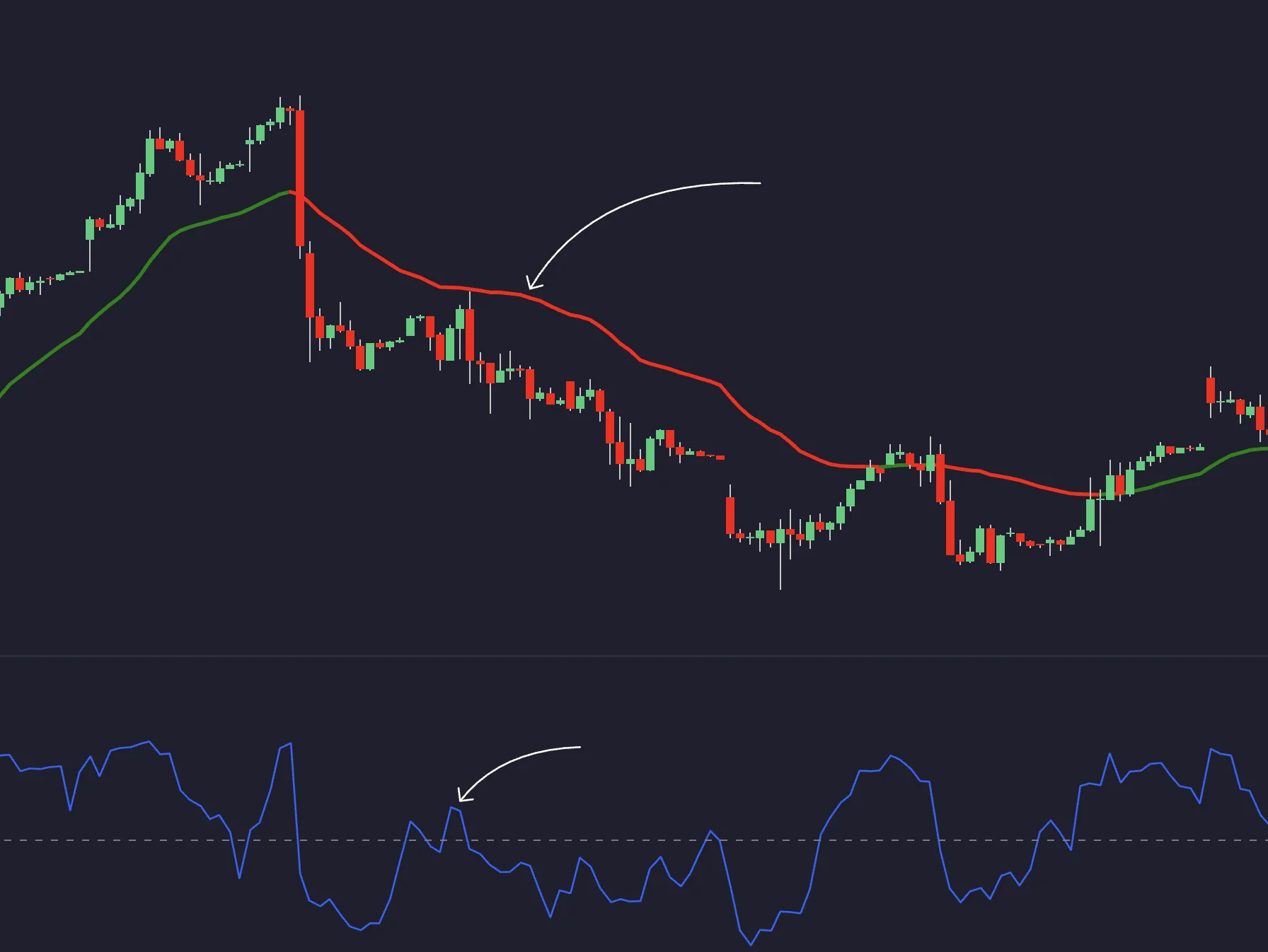
For a selected lookback, let U be the sum of positive close-to-close changes and D the positive magnitude of negative changes. A normalized CMO is (U − D) / (U + D). Its absolute value ranges from zero to one when the denominator is positive. If your indicator reports CMO from −100 to 100, divide by 100 before using it as a smoothing multiplier.
With base EMA length N, the coefficient is a = [2 / (N + 1)] × |CMO|. The recursive update is previous average + a × (current price − previous average). For N = 9 and normalized |CMO| = 0.5, a = 0.1. A previous average of 100 and current price of 110 therefore produce 101.
This formula measures directional imbalance, not simply the size of price movement. Equal upward and downward totals give CMO zero even if those moves are large. A sequence of small moves in only one direction can give an absolute CMO of one. Multiplying every price change by the same positive factor leaves the normalized CMO unchanged.
For the same base N, this coefficient is no larger than the ordinary EMA coefficient. “Adaptive” therefore does not mean “always faster than an EMA.” At CMO zero, the formula retains the previous average. Specify initialization, warm-up data and behavior when U + D is zero; do not let an undefined division silently determine the result.
Choose Periods in Bars, Not Assumed Days
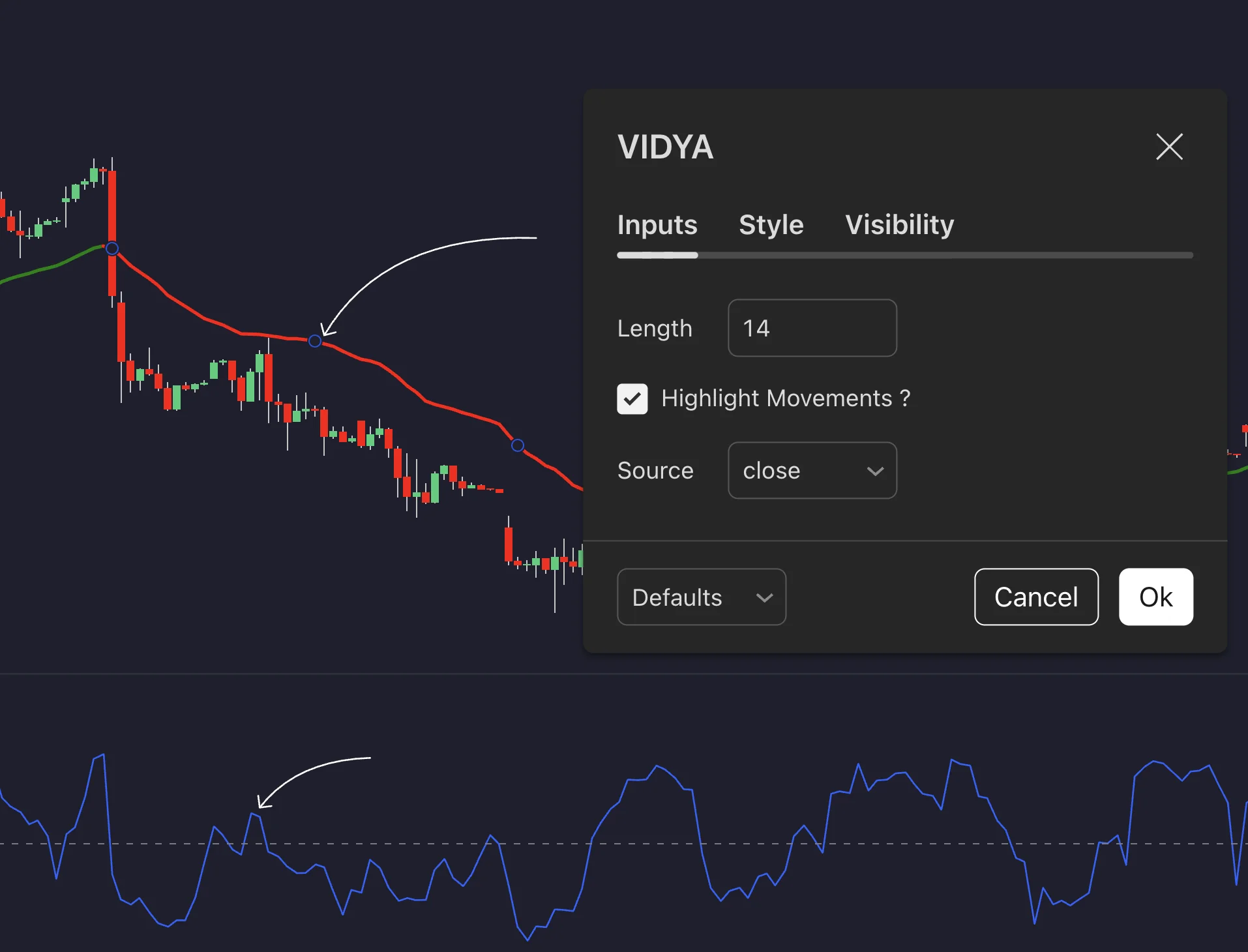
A length of 14 means 14 observations of the selected chart interval. It means days only on an appropriate daily chart. A 14-period average on a fifteen-minute chart and a 14-period average on a daily chart summarize different horizons. An adaptive implementation may have separate lookbacks for the momentum calculation and base smoothing.
Short lookbacks such as 5–20 bars, intermediate lookbacks such as 20–50 bars and longer lookbacks such as 50–200 bars can be research candidates. They are not a universal mapping from high, medium and low volatility to optimal settings. Shortening a lookback in a choppy market may increase turnover; lengthening it may reduce some fluctuations while delaying a genuine change.
A 10-bar adaptive average and a 50-bar average can be assigned different roles, such as a setup condition and broader context. Define those roles before testing. Two lengths on one chart are not the same as two chart timeframes, and their agreement is not independent evidence.
Adjust to a Defined Market Condition
First decide what problem the adjustment is meant to address. Frequent reversals around the average, delayed participation in sustained trends and unexpectedly high trading costs are different observations. Changing settings after each losing trade can fit recent noise rather than improve the method.
- Keep a baseline. Save the current formula, lengths, source price, chart interval, session and complete entry/exit rules.
- Define the condition. If volatility is the trigger, choose a measurement, lookback and threshold using only information available at the decision time.
- Specify the response. State whether the condition changes a coefficient, a lookback, a trade filter or position size. These are different interventions.
- Bound the change. Use explicit minimums, maximums and a review or switching rule; avoid unlimited sensitivity or constant retuning.
- Compare later results. Test the baseline and revision on the same evaluation period with consistent costs, then inspect individual trades and failure cases.
Separate Volatility Bands from Average Sensitivity
Bollinger Bands commonly use a moving-average center with standard-deviation-based bands. Modern Keltner Channels commonly use an EMA center with ATR-based bands. Changing a band multiplier changes the envelope width; it does not automatically change the center average’s smoothing coefficient.
If you want band width or ATR to control an adaptive average, write that mapping explicitly and test it. ATR measures range in price units, while a normalized measure such as ATR divided by price can help compare relative movement across differently priced instruments. A wider band is not evidence of trend direction.
Avoid treating a CMO multiplier, a standard-deviation measurement and an ATR stop distance as interchangeable “volatility settings.” Each measures or controls something different. A faster average may respond to a directional move while a wider adverse-exit distance changes position sizing and execution exposure.
Combine Indicators and Timeframes with a Purpose
An average crossover paired with RSI below 30 is a hypothesis, not automatic confirmation of a rebound. RSI can remain low while price continues falling. Similarly, MACD and a moving average share price inputs, so agreement can repeat information already present in the setup. Test whether an added condition improves net results rather than merely removing unattractive historical trades.
A four-hour context chart, one-hour setup chart and fifteen-minute entry chart can organize analysis. These are illustrative roles, not preferred settings for every volatile asset. Use matching instruments, venues and session conventions where possible, and specify what happens when the conditions disagree.
Respect candle availability. At 10:35, an hourly bar spanning 10:00–11:00 is unfinished. A rule requiring a completed hourly average must use the previous completed hour, not the eventual 11:00 close. A developing-bar rule requires a test that reproduces what was known at 10:35. Higher-timeframe charts summarize overlapping data; they are not independent votes.
Test the Complete Trading System
| Measure | What to inspect | What it does not establish |
|---|---|---|
| Win rate | Profitable closed trades divided by total closed trades, with an explicit breakeven convention | Whether average gains cover losses and costs |
| Maximum drawdown | Largest peak-to-trough equity decline under a stated equity definition | The worst loss the future can produce |
| Profit factor | Gross trading profit divided by the absolute gross trading loss under a stated cost convention | Reliability when there are few trades or no observed losses |
| Trade count and exposure | Number of observations, holding time and overlapping positions | Independence of trades from the same market episode |
Profit factor is undefined or reported as infinite when its loss denominator is zero; that is not proof of a risk-free system. Distinguish closed-trade balance from equity that includes open positions when reporting drawdown. Review costs and individual fills, especially if shorter settings increase trading frequency.
Separate parameter selection from evaluation on later data. Record how many combinations you tried, include both trending and ranging periods where available, and retain losing cases. A parameter that looks best in hindsight may be sensitive to a small change in dates, costs or settings.
Keep Position Sizing Separate from Signal Confidence
Select a planned loss allowance, then calculate size from the adverse-exit distance and value per unit. If an ATR-based distance doubles while the allowance stays the same, the theoretical size halves before costs and size constraints. An average becoming smoother or several indicators agreeing does not justify ignoring this calculation.
For example, a $200 allowance and $2 of planned adverse movement per share imply 100 shares before costs. A $4 distance implies 50 shares under the same assumptions. Stops can fill worse than planned during gaps or fast markets, so this is an estimate rather than a guaranteed loss cap.
Review combined exposure across correlated instruments and avoid increasing size simply because recent trades were profitable. An indicator value is an analytical reference, not a liquidation price or an assurance that an exit will execute there.
Research Adaptive Rules in LuxAlgo’s Native Platform
Use native charts to organize your baseline and comparison views. Check data coverage, chart intervals and session settings before interpreting different average values.
Ask Quant, our coding agent to express a supported version of the formula and complete trade rules. Inspect the generated code and run it manually. Check CMO normalization, separate lookbacks, initialization, zero-movement handling and higher-timeframe timing. Do not assume that an indicator name guarantees the implementation you intended.
Review strategy settings and individual trades with realistic costs and later evaluation data. A generated strategy needs inspection and testing; it is not an already-validated profitable system.
Frequently Asked Questions
Should I shorten a moving average when volatility rises?
Not automatically. A shorter setting responds faster but can increase reactions to reversals and trading costs. Define the problem and compare the change against a saved baseline.
Does VIDYA always use standard deviation?
No. The MetaQuotes implementation discussed here uses normalized absolute CMO to scale an EMA coefficient. Identify the exact implementation rather than relying on the name.
Is CMO the same as volatility?
No. Its normalized formula measures the imbalance between upward and downward changes. Large alternating moves can yield a low absolute value, while small one-direction moves can yield a high value.
Does a length of 14 mean 14 days?
Only on a suitable daily chart. It usually means 14 observations of the selected interval, and an adaptive average may have multiple lookbacks.
Do wider Keltner or Bollinger bands make the average faster?
Changing the band multiplier changes envelope width, not automatically the center average’s smoothing. A rule linking volatility to sensitivity must be specified and tested separately.
Read next