Concept
Gaussian Mixture Models
Gaussian Mixture Models are Machine Learning concepts. The Library holds 1 implementation, a working definition you can pull into Quant.
Top Gaussian Mixture Models indicator
The top custom implementation, built on the original standard Gaussian Mixture Models formula.
1 total
This Gaussian Mixture Models implementation is strategy-ready: open it in Quant, set your rules, and it backtests automatically.
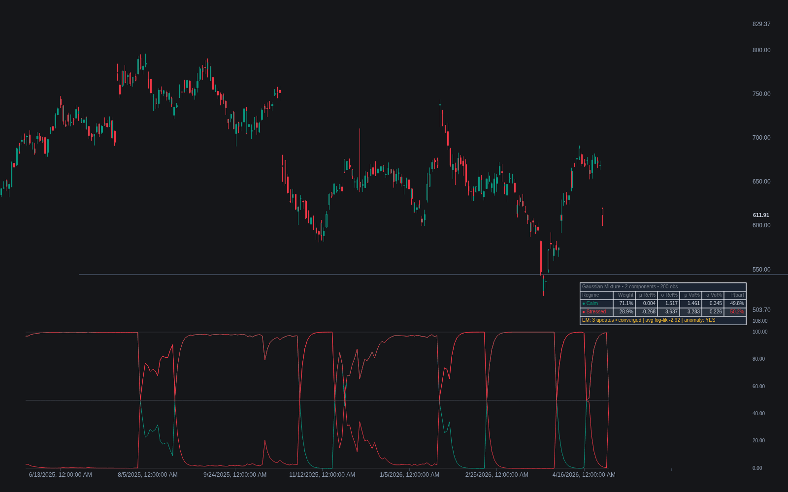
What are Gaussian Mixture Models?
A Gaussian mixture model (GMM) assumes the observed data were drawn from a blend of several normal distributions, each with its own mean, variance (covariance in higher dimensions), and mixture weight. Fitting the model, usually with the expectation-maximization (EM) algorithm, recovers those component parameters and, for every observation, the probability that it came from each component. That soft assignment is the defining feature: rather than declaring a bar a member of the second component outright, a GMM might report 70% odds it belongs to the quiet regime and 30% to the volatile one.
Mixture modeling is one of statistics' oldest ideas: Karl Pearson fit a two-component normal mixture by hand in 1894 to argue that a sample of crab measurements hid two distinct populations. The fitting workhorse arrived in 1977, when Dempster, Laird, and Rubin formalized the expectation-maximization algorithm, the machinery that lets a GMM converge to a fit without needing labeled training data.
In trading, the fitted components double as market regimes. Fit a mixture to features such as returns and volatility and the low-variance component reads as the calm regime, the high-variance component as the stressed one, with the model reporting how confidently the current bar sits in each. It is the probabilistic cousin of K-means regime clustering: where K-means draws hard boundaries around implicitly spherical groups, a GMM fits each component's shape and admits uncertainty. Unlike Hidden Markov / Markov-switching regimes, a plain GMM treats each observation independently, with no memory of which regime came last.
Getting value from a GMM is mostly a data question. Components are only as meaningful as the inputs chosen through feature engineering, and correlated features are often compressed with PCA first so the mixture fits structure rather than redundancy. As a density model it is the parametric counterpart of kernel density estimation, and its posterior probabilities are the currency Bayesian classifiers work in, so regime odds drop straight into probabilistic decision rules.
How to identify GMM output on a chart
A mixture model has no candlestick shape of its own; it shows up through indicators that color bars or plot probabilities by regime.
- 1Add a GMM-based tool such as AlphaNatt's Machine Learning Gaussian Mixture Model and look for regime-colored candles or background shading, sometimes with per-regime probability lines.
- 2Check the settings for the number of components and the input features, most commonly returns and a volatility measure over a training window.
- 3Read the probabilities, not just the colors: values near one mean confident assignment, while middling values mean the bar sits between regimes and labels may flip.
- 4Expect flicker: a plain GMM has no memory, so labels can alternate bar to bar in transitional stretches unless the script smooths the probabilities.
- 5Sanity-check the fit by eye: the high-variance component should coincide with visibly turbulent stretches; if not, the features or component count deserve a second look.
How it's calculated
Models the distribution of a feature such as returns as a weighted sum of K Gaussian components and assigns each observation a probability of belonging to each component.
Shown univariate; the multivariate form replaces μ_k and σ_k^2 with a mean vector and covariance matrix per component.
Fitting uses expectation-maximization from a random or k-means start and can converge to local optima; K is often selected with BIC or AIC.
In market use the fitted components are commonly read as regimes, such as quiet and volatile states.
How traders use it
- As a regime classifier: fit two or three components to volatility and return features, label each bar with its highest-probability component, and gate strategy logic by regime (trend rules in the calm component, mean-reversion or stand-aside in the stressed one), a probabilistic take on volatility regime classification.
- As a distribution model: a mixture of normals reproduces the fat tails and skew that a single bell curve misses, so GMMs appear inside tools that estimate where returns actually concentrate instead of assuming normality.
- As a soft filter: because the output is a probability per regime, signal weight or position size can scale continuously with regime confidence rather than flipping at a hard threshold.
- As an anomaly flag: an observation with low likelihood under every component is unlike anything in the training window, a warning that current conditions may not match the fitted regimes.
- As a pipeline stage: regime probabilities become features or gates for downstream models, blended with other signals through ensemble voting, with the label definition and prediction horizon fixed before judging results.
- On a refit schedule: fits go stale as markets drift, so practical tools refit on a rolling window or update incrementally in the spirit of online learning, accepting that past labels can change with each refit.
GMMs vs adjacent modeling approaches
K-means Regime Clustering: K-means makes hard assignments around implicitly equal, spherical groups; a GMM fits each component's own shape and weight and returns probabilities, at the price of more parameters to estimate.
Hidden Markov / Markov-switching Regimes: An HMM adds a transition matrix, so today's regime depends on yesterday's, giving persistent labels. A plain GMM scores every bar independently, simpler but prone to label flicker in choppy conditions.
Kernel Density Estimation: KDE estimates the distribution nonparametrically with no components at all, flexible but yielding no regime labels. A GMM imposes a few normal components, buying interpretability and probabilities at the risk of choosing the wrong count.
Concept family
Machine Learning
32 concepts mapped · 32 in the Library
Gaussian Mixture Models FAQ
Turn Gaussian Mixture Models into a trading strategy.
Take the implementation from this page into Quant, then build on it, backtest it on real data, and keep refining it in conversation.