How is KDE different from a volume profile histogram?

A histogram splits price into fixed bins, so its shape depends on bin width and where the bin edges fall, and it renders as steps. KDE replaces bins with overlapping kernels centered on each observation, producing one smooth curve free of bin-edge artifacts. Bandwidth takes over the role of bin width: it is the single control that decides how much detail survives smoothing.

What bandwidth should be used for kernel density estimation?

There is no universally correct value. Statistical rules of thumb such as Silverman's rule scale bandwidth to the data's spread and sample size, and charting tools usually expose it as a smoothing input. The practical test is stability: a useful bandwidth keeps the same major peaks when the window shifts slightly, while zones that merge or split with every new bar signal a poor setting.

Does the choice of kernel function matter?

Far less than bandwidth. The classical result is that reasonable kernels (Gaussian, Epanechnikov, triangular) produce nearly identical estimates once bandwidth is tuned, differing mainly in computation and edge behavior. Practical implementations default to the Gaussian for smoothness or the Epanechnikov for efficiency, and no charting decision should hinge on that choice.

Should KDE be applied to prices or returns?

Both, for different questions. Applied to traded prices or volume at price, the density maps where business happened, feeding level work. Applied to returns, it profiles the move distribution, skew, tails, and modes, for risk and threshold calibration. Mixing them up produces nonsense: a price density says nothing about tail risk, and a return density locates no support.

How are KDE peaks used for support and resistance?

A mode in the traded-price or volume-at-price density is a price the market repeatedly accepted, so it is promoted to a support or resistance candidate the same way a high-volume node is. Peak prominence serves as the strength score, and the valleys between modes mark the thin zones where price historically moved fast. The usual level discipline still applies: reaction there is evidence, not entitlement.

When is a Gaussian mixture model better than KDE?

When structure and compactness matter more than fidelity: a mixture summarizes the distribution in a few interpretable components (useful for regime labeling), extrapolates more gracefully in thin samples, and costs less to evaluate. KDE wins when the shape is genuinely unknown and the sample is rich, or when imposing component counts would prejudge exactly the question being asked.

Concept

Kernel Density Estimation

Kernel Density Estimation, also known as KDE, is a Machine Learning concept. The Library holds 2 implementations, each one a working definition you can pull into Quant.

Top Kernel Density Estimation indicators

The top custom implementations, built on the original standard Kernel Density Estimation formula.

2 total

Any of the 2 Kernel Density Estimation implementations below can become a backtested trading strategy — describe your rules and Quant writes the code.

KDE Value Clouds

Indicator

Gaussian Volume Profile

Indicator

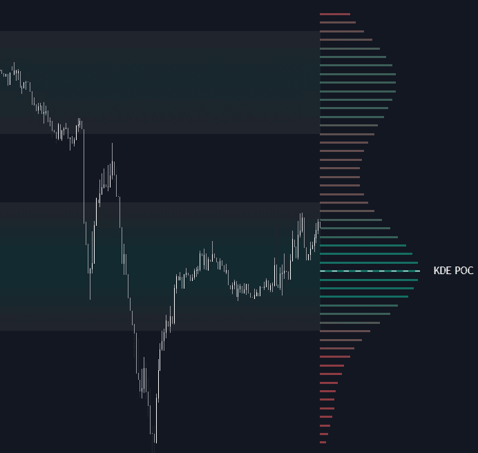
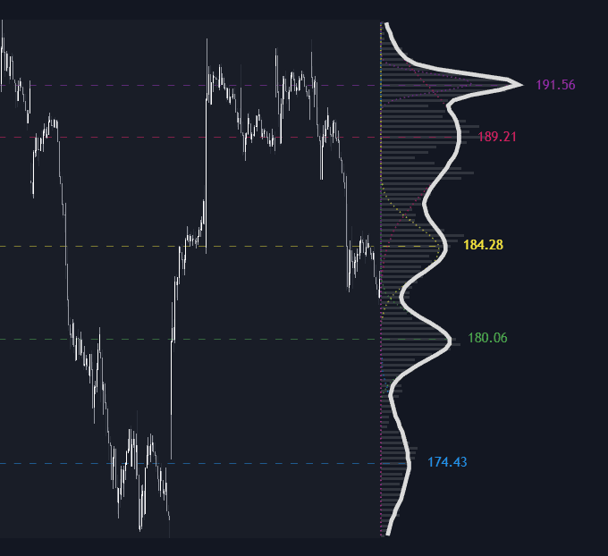
What is Kernel Density Estimation?

Kernel density estimation (KDE) is a nonparametric way to estimate a probability distribution from data without assuming its shape. Each observation contributes a small kernel, commonly a Gaussian bump, centered on its value; summing the bumps and normalizing yields a smooth density curve. A single bandwidth parameter sets how wide each bump is, and therefore how smooth the estimate is: too narrow and the density chases noise, too wide and genuinely distinct peaks merge into one.

The method is a statistics classic, introduced through Murray Rosenblatt's and Emanuel Parzen's work in the 1950s and 1960s (it is still sometimes called Parzen windowing). A standard result of that literature carries straight to charts: the kernel's exact shape matters little, while bandwidth choice matters enormously, which is why rules of thumb such as Silverman's exist and why serious implementations expose bandwidth as the one control worth touching.

On charts, KDE is most often applied to traded prices or volume at price, producing a smooth alternative to the binned histogram of a volume profile. Peaks in the density, its modes, mark prices where activity concentrated and play the same role as high-volume nodes and the point of control; low-density valleys mark prices the market moved through quickly. The same tool is applied to returns to profile their distribution, where skew and fat tails show up directly instead of being assumed away.

Within the machine-learning toolbox, KDE is the nonparametric end of a spectrum. Where a Gaussian mixture model explains data with a few fitted components, KDE spends one bump per observation and lets the sample speak; the same kernels reappear in kernel regression for estimating conditional means, and density estimates feed Bayesian classifiers that need class-conditional likelihoods. Its costs are the usual nonparametric ones: sensitivity to sample size, boundary distortion at the edges of the data, and everything hinging on bandwidth.

How to read a KDE overlay on a chart

KDE renders as a smooth density curve, typically rotated alongside the price axis; the reading is modes, valleys, and stability.

1Identify the input first: a density of traded prices, of volume at price, or of returns are three different objects with different uses.
2Read the modes: local peaks mark values where observations concentrated, the smooth equivalent of high-volume nodes on a profile.
3Read the valleys: low-density stretches mark prices the market rejected or transited quickly, candidate fast-move zones on revisit.
4Judge prominence: a mode's height and isolation grade how dominant that concentration is, which is the rough strength score level-generation uses.
5Test bandwidth stability before trusting zones: nudge the smoothing and keep only the peaks that survive; features that appear and vanish with small bandwidth changes are artifacts.

How traders use it

As a smoothed profile: density peaks locate heavily traded zones and valleys locate low-volume nodes, without the jagged edges and bin-size sensitivity of a histogram.
As level generation: density modes are promoted to support and resistance candidates, with the prominence of each peak used as a rough strength score.
As distribution profiling: applied to returns, the estimated density reveals skew and fat tails that a normality assumption would hide.
As an anomaly gauge: readings that fall in the estimated density's thin regions are outliers by the sample's own account, a nonparametric filter used in feature engineering and signal screening.
As the nonparametric alternative in model choice: when a Gaussian mixture imposes too much shape or too few components, KDE provides the assumption-free baseline the mixture is judged against.

KDE vs related estimation tools

Gaussian Mixture Models: A mixture model fits a small number of parametric components, yielding compact, interpretable structure and hard assumptions. KDE fits nothing: every observation contributes its own bump, so the estimate is flexible, assumption-light, and entirely dependent on bandwidth.

Kernel Regression: Same kernels, different target: kernel regression estimates the conditional mean of one variable given another, drawing smooth curves through scatter, while KDE estimates the distribution of a single variable. One answers where the average is; the other answers where the mass is.

kNN Analog Forecasting: Both are neighborhood methods that let data speak without a fitted formula. kNN queries the k nearest historical analogs for a point forecast; KDE aggregates the whole sample into a density. kNN's bandwidth is its neighbor count, the same smoothing dial wearing different clothes.

Concept family

Machine Learning

32 concepts mapped · 32 in the Library