When is an SVM a reasonable choice for market data?

When the training set is modest and the feature count is high relative to it: the maximum-margin objective plus regularization gives some protection against overfitting, and kernels capture smooth nonlinear boundaries without manual feature crosses. On very large datasets, training cost grows steeply and tree ensembles or neural networks become the more common choice. As always, out-of-sample validation decides.

Does an SVM output probabilities?

Not natively. The raw output is a signed score proportional to the example's distance from the decision boundary: the sign gives the class and the magnitude says how deep in that class's territory the example sits. Converting that score into a probability requires a calibration step such as Platt scaling, which fits a sigmoid to held-out outputs. Calibrate before using SVM scores to size positions.

What is the kernel trick in an SVM?

The optimization only ever uses inner products between examples, so replacing that product with a kernel function makes the model act as if the data lived in a much higher-dimensional space where a flat boundary suffices, without ever computing that space. RBF kernels give smooth local boundaries, polynomial kernels capture interactions, and a linear kernel remains sensible when features are already informative.

What do the C and gamma parameters control?

C prices margin violations: high C chases every training point, tightening the fit and raising overfitting risk, while low C accepts errors for a wider, simpler margin. Gamma, for the RBF kernel, sets each support vector's reach: high gamma makes the boundary local and wiggly, low gamma smooths it out. The two interact, so they are tuned jointly.

Do SVMs overfit financial data?

Any flexible model can. The margin objective and regularization give SVMs some built-in restraint, but noisy labels and shifting regimes defeat a carelessly validated model regardless of algorithm. The defenses are unglamorous: fewer and better features, walk-forward validation instead of shuffled splits, and scheduled retraining as data ages.

Concept

Support Vector Machines

Support Vector Machines are Machine Learning concepts. The Library holds 1 implementation, a working definition you can pull into Quant.

SVM signals

Top Support Vector Machines indicator

The top custom implementation, built on the original standard Support Vector Machines formula.

1 total

The Support Vector Machines implementation below can become a backtested trading strategy — describe your rules and Quant writes the code.

Structural SVM Ranker

Indicator

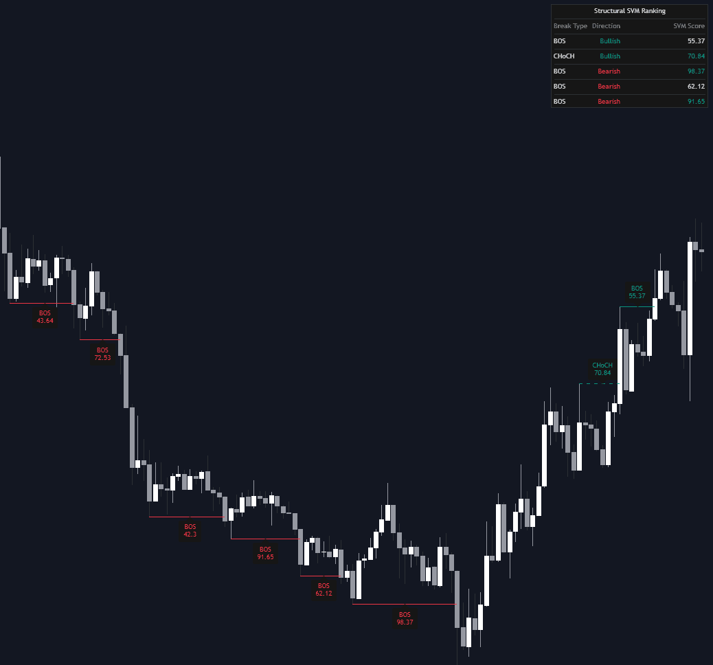
What are Support Vector Machines?

A support vector machine (SVM) is a supervised classifier that separates two classes with the boundary maximizing the margin, the distance to the nearest training points on each side. Those nearest points are the support vectors; they alone determine the boundary, and everything farther away could move without changing it. A regularization parameter (conventionally written C) trades margin width against training errors, and the kernel trick lets the model draw nonlinear boundaries by implicitly working in a higher-dimensional space, with radial basis function (RBF) kernels a common default.

The method grew out of the statistical learning theory that Vladimir Vapnik and Alexey Chervonenkis began developing in the 1960s. Boser, Guyon, and Vapnik presented the kernelized maximum-margin classifier in 1992, and Cortes and Vapnik added the soft-margin form that tolerates misclassified points in 1995. Through the following decade SVMs were among the most widely used classifiers in machine learning, and they remain a common baseline for scarce data even now that neural networks dominate large-scale problems. A sibling formulation, support vector regression (SVR), applies the same margin machinery to continuous targets.

In trading use, an SVM maps a vector of engineered features for each bar or setup into a class defined by the label and horizon: up versus down, trade versus skip, trend versus range. SVMs are historically favored for small-to-medium datasets with many features, where the margin objective provides some built-in resistance to overfitting. The raw output is a score reflecting how far an example sits from the boundary, useful for ranking conviction but not a probability without an explicit calibration step.

Two practical details matter as much as the algorithm. SVMs are geometry-based, so features must share a scale: one large-valued input can dominate the kernel, and redundant inputs distort distances, which is why standardization and sometimes PCA precede training. Markets also drift, and a boundary fit on one regime decays as conditions change, so live use means retraining on rolling windows or switching to online learning rather than fitting once.

How to build an SVM signal model

An SVM leaves no signature on a chart; the craft sits in the pipeline around it.

1Fix the target first: choose the label and horizon, such as the sign of the forward return over N bars, because every downstream choice inherits it.
2Engineer and standardize the features (returns, volatility measures, oscillator readings) so everything sits on a comparable scale.
3Choose a kernel and tune C, plus gamma for RBF, with walk-forward validation rather than shuffled splits, keeping test data strictly in the future.
4Calibrate the margin scores on held-out data if sizing depends on them, then judge the model on out-of-sample results alone.

How traders use it

Directional classification: train on labeled historical bars and take signals only when the model's output clears a margin threshold, so borderline cases are skipped rather than traded.
Setup ranking: because distance from the boundary orders examples by how cleanly they sit in a class, an SVM can rank candidate setups and let only the clearest through a pipeline.
Regime classification: trained on volatility and efficiency features, an SVM can label conditions as trend or range and gate which sub-strategy fires, a supervised counterpart to K-means regime detection.
Trade filtering: a second-stage model predicts whether a base strategy's signals tend to work and vetoes the weak ones, a structure the quantitative literature calls meta-labeling.
Ensemble membership: SVM outputs combine naturally with trees or kNN forecasts in ensemble voting, where disagreement between unlike model families is itself information.
Anomaly screening: the one-class SVM variant learns the envelope of normal conditions and flags bars outside it, useful for standing aside during unusual sessions rather than predicting direction.

SVMs vs adjacent models

kNN Analog Forecasting: kNN keeps the whole training set and votes among the nearest examples at prediction time; an SVM compresses training into a boundary held up by a few support vectors. kNN adapts locally with no training phase, while the SVM generalizes globally and evaluates quickly once fit.

Neural Networks: Neural networks learn their own representations and keep improving with more data, at the price of many design choices and a non-convex fit. SVM training solves a convex problem with a handful of hyperparameters, easier to tune and audit on the small, noisy datasets typical of trading.

Logistic Signal Calibration: Logistic regression produces probabilities natively from a linear boundary; an SVM produces margins and borrows a logistic fit (Platt scaling) when probabilities are needed. Kernels give the SVM nonlinearity a plain logistic model lacks, at some cost in transparency.

Concept family

Machine Learning

32 concepts mapped · 32 in the Library