What is the difference between ACF and PACF?

The ACF at lag k is the plain correlation between the series and itself k bars back, so it includes effects passed along through intermediate lags. The PACF removes those intermediate effects and isolates the direct lag-k relationship. In model identification, a sharp PACF cutoff suggests an autoregressive order, while a sharp ACF cutoff suggests a moving-average order.

What does negative autocorrelation in returns mean?

At the measured lag, up moves have tended to be followed by down moves and vice versa, which is a mean-reversion signature. It is a tendency in that sample, not a rule: the value drifts across regimes, depends on the lookback, and small readings can be indistinguishable from noise without a significance test.

Why do liquid markets show near-zero return autocorrelation?

Because persistent autocorrelation is a free lunch: if today's return reliably predicted tomorrow's, systematic traders would trade it until it faded. What survives is small, unstable, and concentrated where frictions protect it, short horizons, illiquid instruments, stressed regimes. That is also why measured autocorrelation edges deserve skepticism proportional to how easy they would be to arbitrage.

How is autocorrelation significance tested?

The workhorse is the noise band: for a series of length N with no true autocorrelation, sample values mostly fall within roughly plus or minus two over the square root of N, so bars inside that band are unremarkable. Portmanteau tests such as Ljung-Box aggregate across lags. Both assume enough data and reasonably stable conditions, which rolling market samples routinely strain.

Why check squared returns separately?

Because markets hide their memory there. Raw returns can be serially uncorrelated while squared returns correlate strongly for dozens of lags, meaning the size of moves persists even when direction does not. That pattern, the ARCH signature, is the empirical basis for volatility-forecasting models and for treating current volatility as informative about the near future.

What lookback should rolling autocorrelation use?

Long enough for the estimate to mean something, short enough to track regime change: with the noise band scaling as one over the square root of N, windows under a hundred observations produce bands so wide that only large effects register. Common practice runs a few hundred bars for short-lag reads and accepts that the choice, as always, trades statistical power against responsiveness.

Concept

Autocorrelation

Autocorrelation is a Statistics concept. The Library holds 1 implementation, a working definition you can pull into Quant.

ACF/PACF

Top Autocorrelation indicator

The top custom implementation, built on the original standard Autocorrelation formula.

1 total

From studying Autocorrelation to trading it: take the implementation below into Quant and backtest it instantly.

Autocorrelation

Indicator

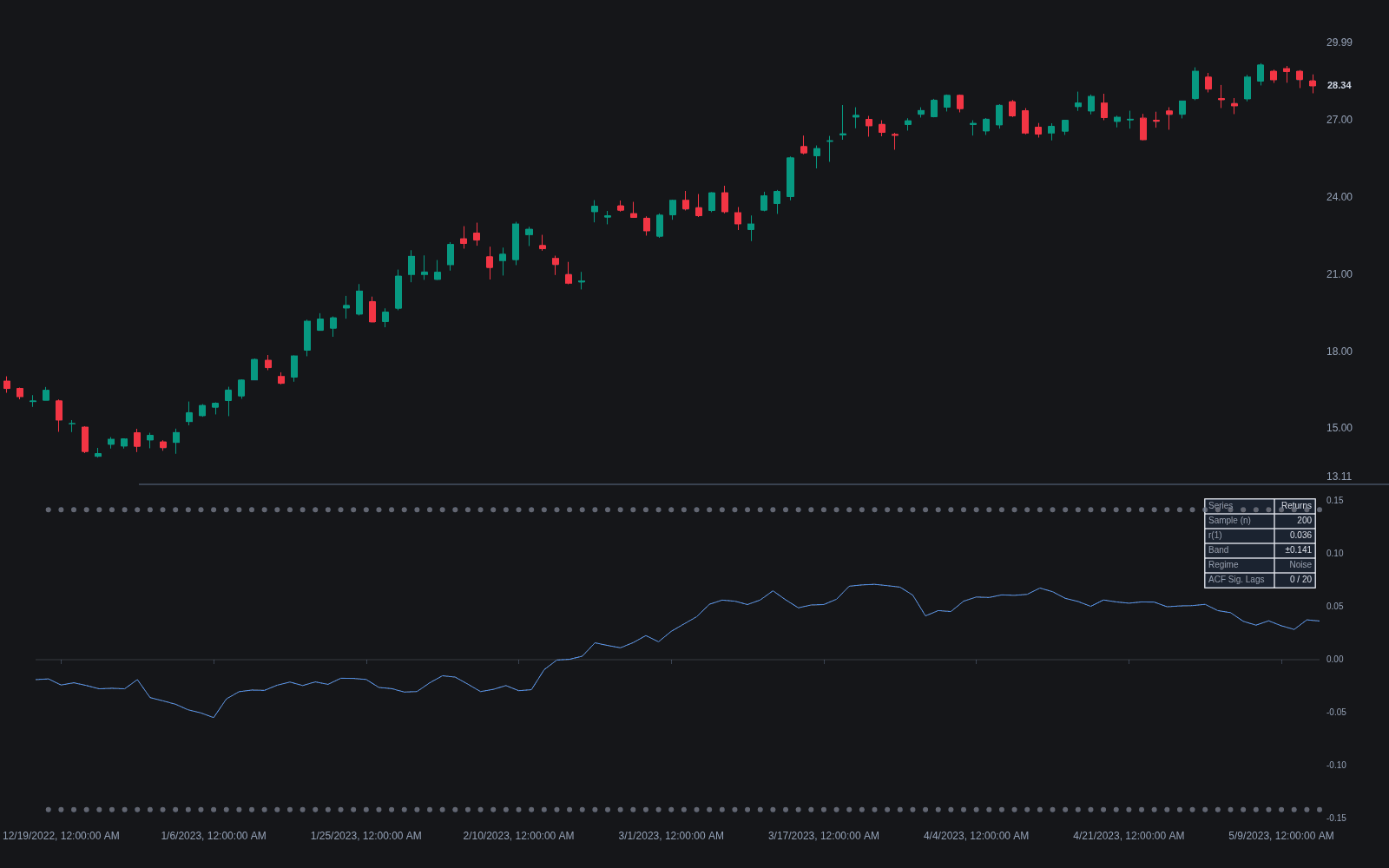
What is Autocorrelation?

Autocorrelation is the correlation of a series with a lagged copy of itself. The autocorrelation function (ACF) reports it across lags: the lag-5 value measures how strongly today's observation moves with the one five bars back. The partial autocorrelation function (PACF) isolates each lag's direct effect by stripping out the influence of shorter lags, which is why the ACF/PACF pair is the classic tool for choosing autoregressive and moving-average orders in forecasting models such as ARIMA.

The machinery is time-series orthodoxy: correlogram reading goes back to the field's foundations, and the Box-Jenkins tradition made ACF/PACF inspection the standard opening move of model building. Finance added its own headline findings, chief among them that liquid-market returns show autocorrelations near zero at most lags (arbitrage eats persistent ones), while the squared and absolute returns stay strongly autocorrelated for long stretches, the statistical signature of volatility persistence.

On returns, autocorrelation is a persistence read: significantly positive values mean moves tend to follow through, negative values mean they tend to snap back, and near-zero is what liquid markets usually show. On price, regular peaks in the ACF at evenly spaced lags reveal cyclicality, the idea behind the autocorrelation periodogram. Like any correlation, the estimate is sample-dependent and drifts across regimes.

Estimation discipline carries the whole exercise. Sample autocorrelations fluctuate even for pure noise, with rough significance bands near two divided by the square root of the sample size, so small readings inside the bands are silence, not signal; regimes drift, so rolling estimates matter more than full-sample ones; and the series choice decides the question asked, returns for direction persistence, squared returns for volatility persistence, price only for cycle hunting after detrending.

How to read autocorrelation on a chart

ACF tools plot bars per lag with significance bands; the reading is sign, lag, and series.

1Fix the input series first: raw returns ask about direction persistence, squared or absolute returns about volatility persistence, detrended price about cycles.
2Plot the ACF with its significance bands (roughly plus or minus two over the square root of the sample size) and ignore bars inside them.
3Read the short lags on returns: positive spikes are momentum-friendly evidence, negative spikes mean-reversion-friendly, at that lag and in that sample.
4Check squared returns separately: long, slowly decaying positive autocorrelation there is volatility persistence, present even when return autocorrelation is nil.
5Use the PACF when model building: its cutoff pattern suggests autoregressive order the way the ACF's suggests moving-average order.
6Re-estimate on rolling windows: the readings drift with regime, and yesterday's persistence signature is not a standing fact.

How it's calculated

Measures how strongly a series correlates with its own past values at a given lag, from -1 (mean-reverting) to +1 (persistent).

m = \frac{1}{N} \times \sum_{t=1}^{N} x_t

\mathrm{num}_k = \sum_{t=k+1}^{N} (x_t - m) \times (x_{t-k} - m)

\mathrm{den} = \sum_{t=1}^{N} (x_t - m)^2

r_k = \frac{\mathrm{num}_k}{\mathrm{den}}

x_t: input series at observation t (for price data, returns are standard, not raw prices)

x_(t-k): the series value k observations earlier

N: number of observations in the sample window

k: lag in observations (k = 1 tests bar-to-bar persistence)

m: sample mean of the series over the window

num_k: lag-k autocovariance sum

den: lag-0 variance sum

r_k: autocorrelation coefficient at lag k, between -1 and +1

t: observation index

Compute on returns rather than raw prices; trending price levels push r_k toward +1 regardless of behavior.

This is the standard estimator; a rolling Pearson correlation of the series against its k-shifted copy differs slightly because each side uses its own mean.

Under a no-correlation null, abs(r_k) above roughly 2 / sqrt(N) is treated as significant.

How traders use it

As a rolling regime gauge: the sign and size of short-lag return autocorrelation helps classify a market as momentum-friendly or mean-reversion-friendly, alongside tools like the Hurst exponent.
For model identification: ACF and PACF shapes suggest how many autoregressive and moving-average terms a forecasting model needs before anything is fit.
For cycle detection: repeating ACF peaks flag a candidate period worth measuring with dedicated cycle tools.
For risk-scaling honesty: serial correlation breaks the independence assumption behind square-root-of-time scaling, so measured autocorrelation corrects volatility annualization and keeps Monte Carlo paths and probability cones from assuming a cleaner world than the data shows.
As a data-quality alarm: strong lag-1 autocorrelation in what should be near-noise returns often flags smoothed, stale, or interpolated data before it flags a tradable effect.

Autocorrelation vs related measures

Correlation: Correlation relates two different series; autocorrelation relates a series to its own past. Same coefficient, different question: co-movement across assets versus memory within one.

FFT/spectral Analysis: The spectrum and the ACF are two views of one object, linked by the Wiener-Khinchin relation: rhythm shows up as evenly spaced ACF peaks in the time domain and as a spectral peak in the frequency domain. Analysts pick the domain that degrades more gracefully on their data.

Fractal Dimension: Fractal dimension (like the Hurst exponent it mirrors) summarizes long-memory roughness in one number; the ACF spreads memory across lags. One is a scalar personality score, the other the full profile it compresses.

Concept family

Statistics

46 concepts mapped · 46 in the Library

Autocorrelation FAQ

Turn Autocorrelation into a trading strategy.

Take the implementation from this page into Quant, then build on it, backtest it on real data, and keep refining it in conversation.

Previous conceptAlpha Next conceptAutocorrelation Periodogram