Monte Carlo Price Paths

What are Monte Carlo Price Paths?

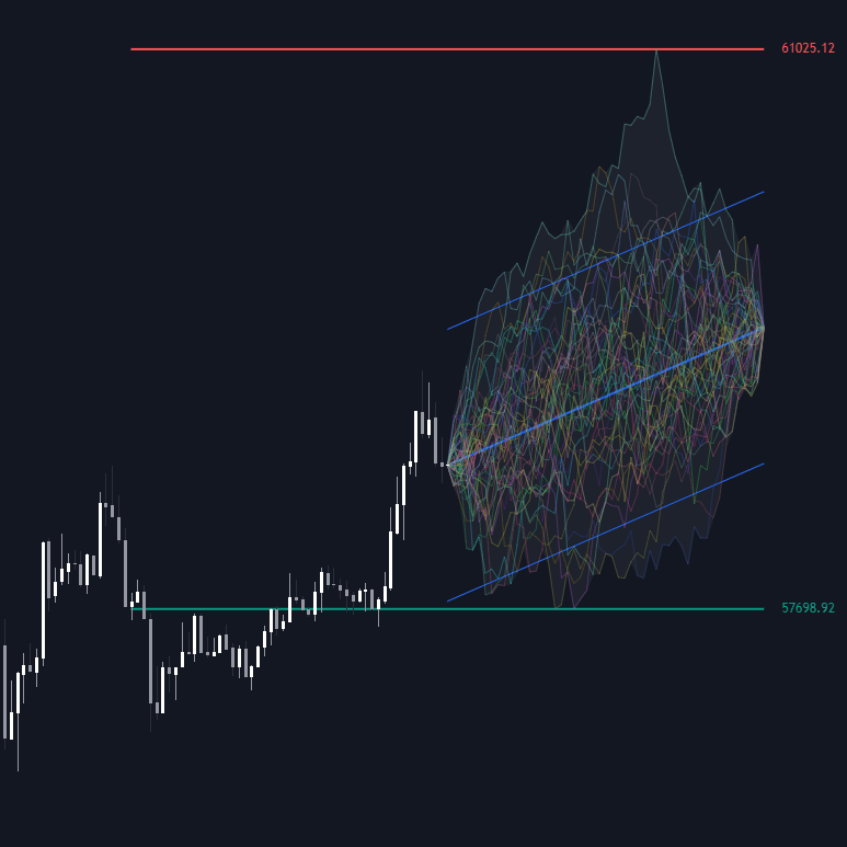
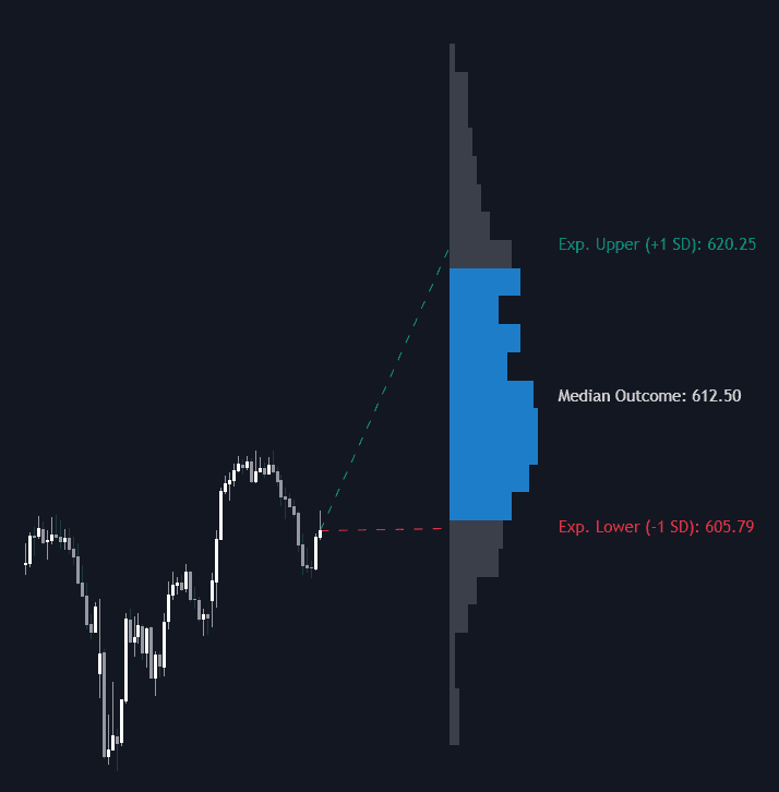
Monte Carlo price paths are simulated futures: many hypothetical forward trajectories generated by drawing random per-bar returns and compounding them from the current price. The draws come either from a fitted model (a drift and a volatility, often estimated from recent realized volatility, driving a geometric random walk) or from bootstrapping, meaning resampling or shuffling the instrument's own historical returns. No single path is a forecast. The information lives in the ensemble: percentile envelopes, the distribution of terminal prices, and frequencies such as the share of paths that touch a level within the horizon.

The method itself is mid-century physics: Stanislaw Ulam and John von Neumann developed Monte Carlo simulation for nuclear calculations in the 1940s, and finance adopted it in stages, from Phelim Boyle's 1977 use in option pricing to the risk engines and retail charting tools of later decades. The trading application inherits the original premise unchanged: when a system is too messy to solve analytically, simulate it many times and read the distribution of outcomes.

A second flavor, trade-sequence Monte Carlo, applies the same idea to a strategy instead of a market: reshuffling or resampling the order of historical trades shows the range of equity curves and drawdowns the same trade population could have produced. Both flavors inherit their assumptions. Independent draws ignore volatility clustering and autocorrelation, so standard implementations tend to understate how extreme and how clustered real moves can be.

The craft is in the generator. Model-based paths (drift plus volatility) are transparent but Gaussian-thin in the tails; simple bootstrapping keeps the observed distribution's shape, including its skew and fat tails, but scrambles the time structure; block bootstrapping resamples runs of consecutive returns to preserve some autocorrelation and clustering. Whichever generator is chosen, the ensemble is a statement of the assumptions, which is why serious use starts from a measured return profile rather than defaults.

How to read a Monte Carlo projection on a chart

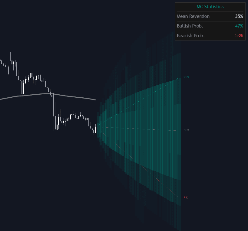
Monte Carlo overlays render as path fans or percentile envelopes projected from the current bar; the reading discipline is about the ensemble, never the strands.

1. 1Check the generator first: a drift-and-volatility model, an IID bootstrap, or a block bootstrap produce differently shaped fans from the same history.
2. 2Read the percentile envelope, not individual paths: the bands state where the stated fraction of simulated futures remained, under the assumptions.
3. 3Use the terminal distribution for horizon planning: its spread and skew describe the range of end states the generator considers plausible.
4. 4Read touch frequencies where offered: the share of paths reaching a stop or target within the horizon is the simulation's answer to a trade-planning question.
5. 5Rerun before trusting: if the statistic you care about shifts materially between batches, the run count is too small for that statistic.
6. 6Distrust the extreme tails on principle: independence assumptions understate clustered, violent sequences, so real markets escape simulated ranges more often than the labels imply.

How traders use it

• To draw forward scenario envelopes: percentile bands over the simulated ensemble form probability cones that frame how far price could plausibly travel within a horizon under the stated volatility.
• To estimate level-touch odds: the fraction of paths that reach a stop or target within N bars serves as a rough, assumption-dependent probability for trade planning.
• To stress a backtest: shuffling trade order, one of the standard resampling tests, reveals how much of the realized drawdown was sequence luck and what worse orderings look like.
• To size soberly: the simulated drawdown distribution, rather than the single historical drawdown, sets risk budgets, since the one path history happened to print is just one draw from the ensemble.
• To score outcomes after the fact: locating the realized move as a percentile of the simulated distribution turns 'was that normal?' into a number, the simulation-based cousin of a z-score surprise reading.

Monte Carlo paths vs related projection tools