Distribution Moments

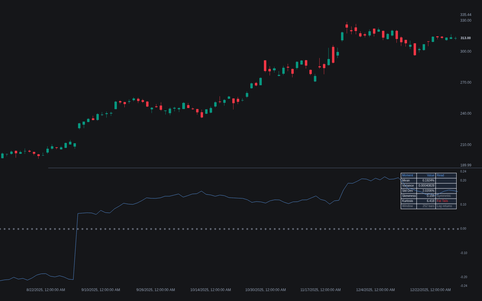
What are Distribution Moments?

Distribution moments are the statistics that summarize the shape of a return distribution. The first moment is the mean; the second central moment is variance, whose square root is standard deviation. The third standardized moment is skewness, which measures asymmetry: negative skew means a longer left tail, so the outsized surprises tend to be downside. The fourth standardized moment is kurtosis, which measures tail weight; a normal distribution has kurtosis of 3, and readings above that (positive excess kurtosis) are the usual quantitative marker of fat tails. Standardized means each is divided by the matching power of standard deviation, so skewness and kurtosis are unitless shape numbers.

The machinery is classical statistics: moment-based description of distributions was systematized by Karl Pearson's work in the late nineteenth century, long before finance adopted it. Markets forced the adoption. Benoit Mandelbrot's 1963 study of cotton prices famously documented tails far heavier than the normal model allows, and decades of subsequent research have confirmed heavy tails and asymmetry as standing features of speculative returns rather than curiosities.

They matter because market returns are not normal. Equity index returns typically show negative skew and clear excess kurtosis, so tools that assume normality, such as z-score thresholds and sigma-multiple bands, understate how often extreme moves occur. Profiling the moments of the actual data (see distribution-of-returns profiling) shows how far those assumptions can be trusted on the market at hand.

The estimation caveat is severe for the higher moments. Skewness and kurtosis are powered by cubed and fourth-powered deviations, so a single outlier can dominate an entire window's estimate, and rolling readings jump when that outlier enters or exits the sample. Short windows produce numbers too noisy to trust, which is why practitioners lean on long samples, report alongside a percentile rank view of the same data, or use robust alternatives when the sample is thin.

How to read moment gauges on a chart

Moments appear on charts as rolling-window panes; reading them is mostly about respecting their estimation noise.

1. 1Fix the inputs: a return series (log or simple) and a window long enough for the moment you want, with higher moments demanding much more data.
2. 2Read rolling skewness by sign and persistence: a stretch of negative readings says recent surprises lean downside; single-bar flips mean little.
3. 3Read kurtosis against 3 (or excess kurtosis against 0): persistently elevated readings mark a tape whose extremes outrun sigma-based expectations.
4. 4Trace spikes to their cause before believing them: one outlier bar entering the window can swing both higher moments dramatically, and the reading will jump again when it leaves.
5. 5Cross-check against a nonparametric view, such as the return histogram or percentile table, before letting a moment reading change risk decisions.

How it's calculated

Skewness and kurtosis standardize the third and fourth central moments of returns, measuring the asymmetry and tail weight of the distribution.

A normal distribution has Skew = 0 and Kurt = 3; positive excess kurtosis signals fat tails, and negative skew a heavier downside, both typical of equity returns.

These are the population estimators; sample versions apply bias corrections such as the n - 1 variance denominator and the Fisher-Pearson adjusted skewness.

Compute the moments on returns rather than raw prices, since prices are non-stationary.

How traders use it

• As a rolling risk read: tracking skewness and kurtosis over a moving window can flag a deteriorating tail environment even while realized volatility still looks calm, though higher-moment estimates are noisy on short windows.
• For threshold calibration: high kurtosis argues for empirical cutoffs such as percentile rank instead of sigma multiples, because sigma-based limits are breached more often than normal math implies.
• For instrument comparison: skew separates markets that grind up and crash down from roughly symmetric ones, which informs asymmetric stop and target placement.
• As simulation inputs: Monte Carlo path engines built on normal draws inherit the normal model's thin tails, so moment estimates (or resampling from the empirical distribution) are what make simulated risk resemble the market's actual behavior.
• For projection honesty: probability cones and similar forward bands widen correctly only when the generating assumptions carry the observed skew and tail weight rather than textbook symmetry.

Distribution Moments vs related statistics