Distribution-of-returns Profiling

What is Distribution-of-returns Profiling?

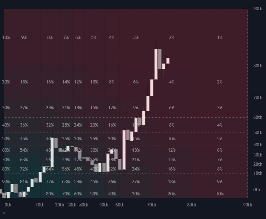
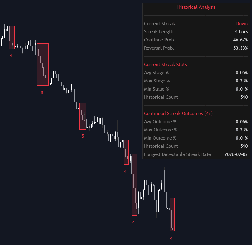
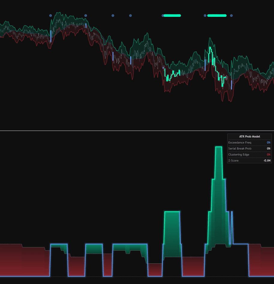
Distribution-of-returns profiling builds the empirical distribution of a market's moves from history and reads its shape directly, instead of assuming a bell curve. Collect returns per bar, per session, or per week, optionally conditioned on context such as weekday or regime, then examine the histogram and its summary statistics: center, spread, skew, and tail weight, the classic distribution moments, along with percentiles and exceedance frequencies such as the share of days that travel more than a given distance.

The workflow has a few load-bearing choices. The return unit sets the question (per-bar returns profile noise, per-session returns profile the tradable day, weekly returns profile the swing horizon); log returns are standard for their additivity, though simple returns read more naturally; and conditioning splits, by session, weekday, or volatility state, turn one anonymous distribution into several answerable ones. Exceedance tables and percentile grids are the usual outputs because they translate directly into trade language: how often does a day travel this far?

The exercise matters because market returns are famously non-Gaussian: fat tails and volatility clustering make extreme moves far more common than a normal curve implies. Profiling the observed sample grounds targets, stops, and expectations in measured frequencies rather than idealized math, and it supplies the raw material for tools such as probability cones and exceedance tables. The estimates are only as good as the sample: tails need a lot of data, and old regimes may not represent current ones.

The pitfalls are the flip side of the power. Markets are not stationary, so a profile spanning a regime break averages two different markets into one misleading picture; every conditioning split thins the sample, and enough splits will find a flattering slice by chance. Serial dependence complicates the story further, since returns that echo their own past (see autocorrelation) make independent-draw reasoning too optimistic. Good profiling reports sample sizes, tests slices out of sample, and treats the result as a description of the past rather than a promise.

How to read a returns-profile tool

Profile tools render as histograms, percentile grids, or probability tables; the reading discipline is the same for all of them.

1. 1Check the definition first: which return unit (bar, session, week), log or simple, and over what sample span; nothing else means anything without these.
2. 2Read the histogram against its fitted normal overlay, if shown: extra mass in the tails and asymmetry between the sides are the non-normality that sigma reasoning misses.
3. 3Read the percentile grid for the market's vocabulary: the median day, the quartile day, the worst-decile day, each in the instrument's own units.
4. 4Use exceedance rows as frequency statements: the share of sessions traveling beyond a given multiple of ATR or percentage tells you how rare a target or stop distance really is.
5. 5For conditioned views, check the per-slice sample size before trusting any difference between slices; thin slices produce loud, meaningless contrasts.

How traders use it

• To size targets and stops from observed frequencies: if only a small share of sessions travel beyond some multiple of ATR, a target parked past that distance is, by the data's own account, a low-frequency outcome.
• To test for conditional edges: split the sample by session, weekday, or volatility regime and compare the distributions; a bias that survives the split, with adequate sample size in each slice, is worth further study.
• To sanity-check model assumptions: comparing the sample's tails against a fitted normal curve shows how badly sigma-based bands and thresholds will understate extremes before you rely on them.
• To choose normalizations: whether a z-score is honest or a percentile rank is required is itself a profiling question, answered by how non-normal the measured distribution turns out to be.
• To feed simulations: resampling from the empirical distribution, or fitting one that matches its moments, gives Monte Carlo paths and probability cones the market's actual tail behavior instead of textbook tails.

Profiling vs related statistical tools