Concept
Hodrick-Prescott Filter
Hodrick-Prescott Filter is a Statistics concept. The Library holds 1 implementation, a working definition you can pull into Quant.
Top Hodrick-Prescott Filter indicator
The top custom implementation, built on the original standard Hodrick-Prescott Filter formula.
1 total
The Hodrick-Prescott Filter implementation below can become a backtested trading strategy — describe your rules and Quant writes the code.
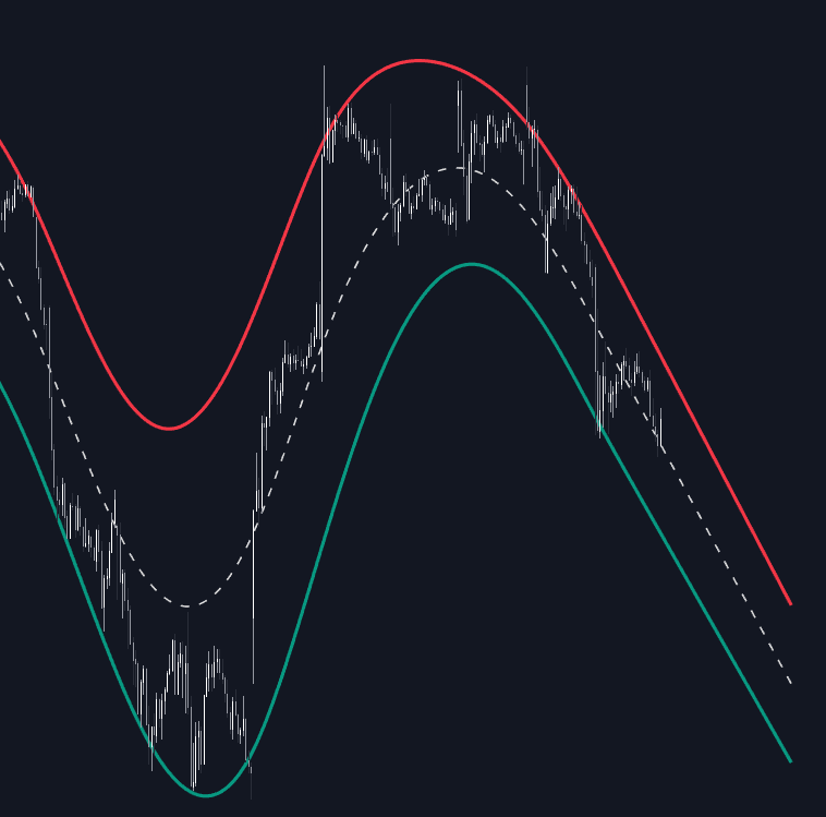
What is the Hodrick-Prescott Filter?
The Hodrick-Prescott (HP) filter is a trend-extraction method from macroeconometrics, introduced to economics by Robert Hodrick and Edward Prescott for separating business-cycle fluctuations from long-run growth. It chooses the trend that minimizes a two-part objective: the sum of squared gaps between the series and the trend (fit), plus lambda times the sum of squared second differences of the trend (a penalty on changes in its slope). Small lambda lets the trend hug the data; as lambda grows the trend stiffens, approaching a straight line in the limit. Mathematically it is a special case of the earlier Whittaker-Henderson smoother with a second-difference penalty.
On charts the filter splits price into a smooth trend and a cycle residual, and adaptations draw envelopes around the smooth to frame stretch and reversion. The critical caveat for trading is that the standard filter is two-sided: each point's trend value is fitted using data on both sides of it, so values near the right edge revise as new bars arrive. Endpoint distortion is a standard criticism in the economics literature as well, and on a chart it means naive use repaints; one-sided (causal) variants avoid revision at the cost of extra lag.
Lambda is the filter's one real decision. Macroeconomists settled on 1600 for quarterly data, and the Ravn-Uhlig rule scales that convention across observation frequencies by the fourth power of the frequency ratio, giving about 129,600 for monthly series. No such convention exists for market bars, so chart implementations expose lambda as an input. Useful practice is to tune it once until the cycle residual oscillates cleanly around zero at the horizon you trade, then freeze it, since a lambda re-tuned per chart is a curve fit waiting to happen.
The filter also carries serious academic criticism worth knowing. James Hamilton's widely cited 2018 paper argued that the HP filter can manufacture spurious cycles, distorts endpoints and rests on an arbitrary lambda, recommending regression-based alternatives; earlier work by Cogley and Nason raised related concerns about spurious dynamics. For chart use the lesson is proportion: treat the output as a descriptive smooth, implemented causally when traded, for example via the one-sided variant computed with a Kalman filter recursion. LuxAlgo's Whittaker Envelope applies the same penalized-smoothing idea with bands added for reversion framing.
How to identify the Hodrick-Prescott filter on a chart
An HP trend looks like a suspiciously smooth moving average with no lag through the middle of history. The tells are at the edges.
- 1Set lambda for your bar frequency and horizon: larger values stiffen the trend toward a line, smaller values let it chase price; tune once on history and freeze it.
- 2Plot the trend and its cycle residual, price minus trend; a well-tuned residual oscillates around zero without long one-sided stretches.
- 3Watch the right edge as new bars arrive: the last stretch of the trend visibly bends and re-settles, which is the two-sided revision in action.
- 4For anything live, switch to a one-sided variant or act only on values old enough to have stabilized, and label the chart accordingly.
- 5Standardize the residual with a z-score if you want comparable stretch readings across symbols and volatility regimes.
How it's calculated
Decomposes a series into a smooth trend and a cyclical remainder by penalizing changes in the trend's slope.
Standard λ values follow the Ravn-Uhlig fourth-power rule: 6.25 annual, 1600 quarterly, 129600 monthly; daily bars need far larger values.
The minimization solves a sparse linear system over the whole sample in one pass.
The filter is two-sided, so recent values revise as new bars arrive; treat the latest stretch as provisional in live use.
How traders use it
- Trend-cycle decomposition: subtract the HP trend from price to get a detrended oscillator around zero, a simple entry point into signal decomposition and cycle study.
- Envelope construction: offset bands around the HP trend (by a volatility unit or a fixed percentage) to frame overextension and mean-reversion zones with a smoother midline than a moving average.
- Higher-timeframe bias reference, provided the two-sided revision is handled honestly: evaluated on confirmed history, replaced with a one-sided variant, or treated as descriptive rather than tradable, in line with repaint-safe engineering.
- Residual mean-reversion study: the z-scored cycle component becomes a stretch oscillator with entry and exit thresholds, effectively a statistically dressed version of trading distance from a smooth midline.
- Research benchmark: because the two-sided fit is close to an ideal smooth on past data, it serves as the reference other causal smoothers are judged against when quantifying how much lag and noise they add.
HP filter vs other trend extractors
Linear Regression: A regression line forces one slope across the window; the HP trend bends wherever the penalty allows, following slow curvature a line cannot. Both are in-sample fits whose newest values revise, but the regression's rigidity makes it more transparent.
Kalman Filter: The Kalman filter is causal and never repaints: each estimate uses only past data, at the cost of lag and an explicit model. The standard HP filter is two-sided and revises; its one-sided variant is in fact usually computed with a Kalman-style recursion.
Exponential Smoothing: Exponential smoothing is a one-pass causal filter with lag proportional to its smoothing constant. The HP filter buys its superior in-sample smoothness by using future data at every interior point, which is exactly what a live chart lacks at the right edge.
Concept family
Statistics
46 concepts mapped · 46 in the Library
Hodrick-Prescott Filter FAQ
Turn Hodrick-Prescott Filter into a trading strategy.
Take the implementation from this page into Quant, then build on it, backtest it on real data, and keep refining it in conversation.