ARIMA Forecasts
ARIMA Forecasts, also known as ARIMA, Box-Jenkins forecasting, autoregressive integrated moving average, ARMA, are Statistics concepts. The Library holds 1 implementation, a working definition you can pull into Quant.
Top ARIMA Forecasts indicator
The top custom implementation, built on the original standard ARIMA Forecasts formula.
1 total
From studying ARIMA Forecasts to trading it: take the implementation below into Quant and backtest it instantly.
What are ARIMA Forecasts?
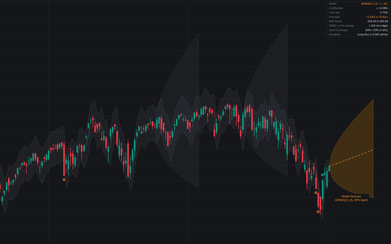
ARIMA forecasts project a series forward with an autoregressive integrated moving-average model, drawn on a chart as a forecast path with prediction bands that widen with the horizon. The series is first differenced d times to remove trend (the integrated part); the differenced values are then modeled as a linear function of their own last p values (the autoregressive part) and the last q forecast errors (the moving-average part, unrelated to a charting moving average). The model is written ARIMA(p, d, q).
George Box and Gwilym Jenkins systematized the method in Time Series Analysis: Forecasting and Control (1970). Their three-stage cycle is still the standard workflow: identify candidate orders from the autocorrelation and partial autocorrelation of a stationary series, estimate the parameters, then check that the residuals look like white noise (for example with the Ljung-Box test). Modern software automates the order choice with information criteria such as AIC, as in Rob Hyndman and Yeasmin Khandakar's auto.arima (2008).
On price charts the honest result is usually modest. Log prices typically need one difference, and returns in liquid markets carry little linear autocorrelation, so fitted models often sit close to ARIMA(0,1,0), the random walk: a flat forecast at the last price (sloped if a drift is fitted) with bands widening with the square root of the horizon. The bands often say more than the center line. The model also assumes constant variance, so with volatility clustering and fat tails its bands run too narrow in turbulent regimes and too wide in quiet ones.
How it's calculated
Difference the series, fit a linear ARMA equation to the result, then iterate it forward with future shocks set to zero.
Parameters are estimated by maximum likelihood; orders come from ACF/PACF reading or from minimizing an information criterion such as AIC.
Once h exceeds q the MA terms drop out; with d = 1, σ_h keeps growing with h, while a stationary series (d = 0) reverts to its mean and σ_h levels off.
Bands assume normal, constant-variance errors. When y is log price, exponentiating the band gives asymmetric price bands.
How traders use it
- As a forecast cone: the h-step bands drawn ahead of price act as a model-based dispersion envelope, the parametric cousin of probability cones, for judging how unusual a later move is.
- As a benchmark: comparing out-of-sample errors against the plain random walk shows whether any linear structure exists, and on most liquid price series the random walk is hard to beat. The test only counts on data the fit never saw (see in-sample / out-of-sample splits).
- On series with more memory than returns: spreads, volume and volatility measures often carry real autocorrelation, so ARIMA earns its keep there more than on raw price, for example on the spread in a pairs trade.
- As a surprise gauge: the one-step forecast error divided by its standard error turns each new bar into a measured surprise.
ARIMA vs related forecasting tools
Exponential Smoothing Forecasts: Close relatives: simple exponential smoothing gives the same forecasts as an ARIMA(0,1,1), and Holt's linear method corresponds to an ARIMA(0,2,2). Smoothing is specified by level, trend and season; ARIMA by the series' correlation structure.
Autocorrelation: Autocorrelation is the diagnostic; ARIMA is the model built on it. The ACF and PACF suggest the orders, and leftover autocorrelation in the residuals says the fit missed something.
GARCH-family Clustering: ARIMA models the conditional mean and assumes constant variance; GARCH models the conditional variance. Combined ARIMA-GARCH fits use one for the forecast path and the other for the width of its bands.
Concept family
Statistics
45 concepts mapped · 45 in the Library
ARIMA Forecasts FAQ
Turn ARIMA Forecasts into a trading strategy.
Take the implementation from this page into Quant, then build on it, backtest it on real data, and keep refining it in conversation.