GARCH-family Clustering

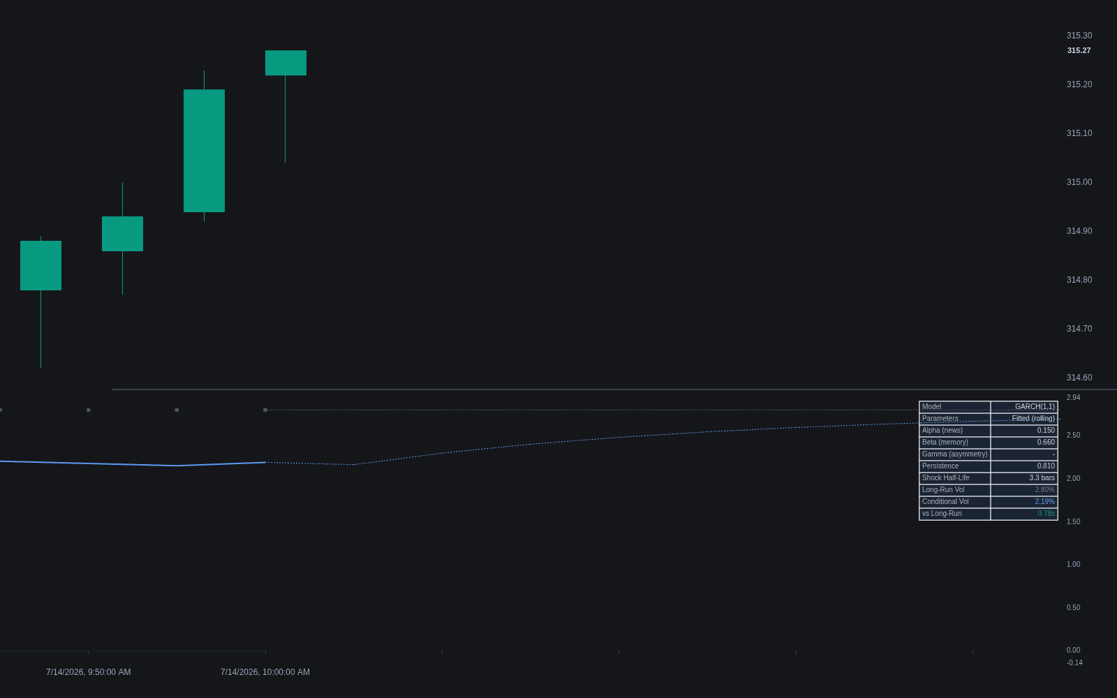
What is GARCH-family Clustering?

GARCH-family clustering refers to modeling volatility clustering, the well-documented tendency of large returns to follow large returns and calm to follow calm, with GARCH models: generalized autoregressive conditional heteroskedasticity, introduced by Tim Bollerslev as a generalization of Robert Engle's ARCH. In the workhorse GARCH(1,1), the next period's conditional variance is a weighted sum of three terms: a constant anchoring the long-run variance, the most recent squared return (the news or shock term), and the previous conditional variance (the persistence term). The sum of the news and persistence weights measures how slowly shocks decay: the closer it sits to one, the longer elevated volatility lingers, and forecasts mean-revert toward the long-run level.

The lineage is unusually well documented for a trading concept. Benoit Mandelbrot described the phenomenon in 1963, observing that large price changes tend to be followed by large changes, of either sign, and small changes by small. Robert Engle formalized it with the ARCH model in 1982, work that earned him a share of the 2003 Nobel Memorial Prize in Economic Sciences, and Tim Bollerslev generalized it to GARCH in 1986. J.P. Morgan's RiskMetrics system later spread the exponentially weighted special case across bank risk desks in the 1990s, which helped make conditional-variance thinking standard in risk management.

Extensions target asymmetry. EGARCH (Nelson) models the logarithm of variance, which removes positivity constraints and lets negative returns raise expected volatility more than equal-sized positive ones, the leverage effect. GJR-GARCH (Glosten, Jagannathan, and Runkle) achieves similar asymmetry with an extra term that activates only after negative returns. Relative to simple realized volatility measurement, the family trades transparency for a model that forecasts rather than merely describes.

For chart-focused traders, the family matters less as something to fit and more as the theory underneath familiar tools. The persistence GARCH estimates is the reason Bollinger Bands stay wide for stretches after a shock, why ATR readings trend rather than jump around randomly, and why squeeze setups exist at all: quiet conditions persist until they break, the observation behind the volatility contraction pattern and squeeze logic generally. GARCH adds two things the chart proxies lack: an explicit long-run anchor that forecasts revert toward, and a fitted estimate of how fast that reversion happens.

How to recognize volatility clustering on a chart

Fitting the models is an off-chart exercise, but the behavior they capture is visible with ordinary tools.

1. 1Plot a rolling volatility proxy beneath price: ATR, realized volatility, or Bollinger BandWidth. Clustering shows up as long quiet stretches and distinct stormy episodes rather than a random mix of bar sizes.
2. 2Look for persistence after shocks: following a news bar or a large gap, elevated ranges linger for days or weeks and taper gradually, which is the decay signature the models parameterize.
3. 3Place the present against history: a volatility percentile reading shows whether current conditions are stretched relative to the instrument's own past, and clustering implies such readings drift back rather than snap back.
4. 4Check the asymmetry in equities: sell-offs typically expand volatility more than rallies of the same size, the leverage effect that EGARCH and GJR-GARCH exist to encode.

How it's calculated

A conditional-variance model that forecasts each bar's variance from a constant, the previous squared shock, and the previous variance, so large moves tend to follow large moves.

Parameters are estimated by maximum likelihood over the return history, not set by hand.

EGARCH models ln(σ_t^2) and GJR-GARCH adds an extra weight on squared negative shocks; both capture the asymmetry where downside moves raise volatility more than upside moves.

α + β near 1 means volatility shocks decay slowly, and the multi-step forecast reverts toward V_L at rate (α + β) per step.

How traders use it

• For forecasting: a fitted model produces multi-step variance forecasts that decay toward the long-run average, a common input to volatility-aware position sizing and stop distances.
• For regime context: comparing current conditional volatility with the model's long-run level separates calm from stressed conditions more formally than eyeballing a chart, one route into volatility regime classification.
• As a benchmark: EWMA volatility is the boundary case with no long-run anchor, so running both shows how much mean reversion in volatility the data actually supports.
• For channel and stop calibration: conditional variance can stand in for the rolling standard deviation or ATR inside band constructions, an alternative engine for the jobs Keltner Channels and similar envelopes usually do with simpler inputs.
• For squeeze context: when a TTM Squeeze or Bollinger squeeze signals compression, a fitted model's persistence and long-run variance give a principled baseline for how unusual the quiet is and how quickly expansions on that instrument have historically decayed.

GARCH-family models vs other volatility measures