Does the Whittaker–Henderson smoother repaint?

The most recent portion does. Because each output point uses data on both sides of it, the newest values are provisional and shift as bars arrive, settling only once enough later data surrounds them. Sections deep inside the window are stable. Signal logic built on the fresh end therefore needs repaint-aware handling or an evaluation delay.

How is Whittaker–Henderson smoothing different from a moving average?

A moving average is causal: each value is a weighted sum of past bars only, which is stable but lagged. Whittaker–Henderson solves for the entire smoothed series at once by penalizing roughness, so interior values use future as well as past data and show almost no lag. The price is end-point instability, whereas a moving average's plotted history never revises.

What does the lambda parameter control?

Lambda weights the roughness penalty against fidelity to the data. Small values track price closely and stay wiggly; large values give a stiffer curve, approaching a straight line under a second-order penalty. There is no universal value; choose by eye or by testing against the timeframe's noise.

Is the Whittaker–Henderson smoother the same as the Hodrick-Prescott filter?

The Hodrick-Prescott filter is the special case with a second-order difference penalty, applied to macroeconomic series. Whittaker–Henderson is the general construction: any penalty order, any lambda, any equally spaced series. With a second-order penalty and the same lambda, the two produce the same curve.

Can I trade signals directly from the smoother?

Not naively. Slope flips and price crossings at the fresh end are computed on values that will revise, so a backtest reading them as fixed overstates results. Workable approaches wait out a confirmation delay, or use the curve for context while timing entries with non-repainting tools such as a Supertrend flip or moving average crossovers.

Which difference order should I use?

Second order penalizes changes in slope and is the standard choice, matching the Hodrick-Prescott filter. Third order allows smooth acceleration, following curved trends with less distortion but reacting a bit more to noise. For most charting the difference is subtle next to the choice of lambda.

Concept

Whittaker–Henderson Smoother

Whittaker–Henderson Smoother is a Trend concept. The Library holds 1 implementation, a working definition you can pull into Quant.

Top Whittaker–Henderson Smoother indicator

The top custom implementation, built on the original standard Whittaker–Henderson Smoother formula.

1 total

The Whittaker–Henderson Smoother implementation below can become a backtested trading strategy — describe your rules and Quant writes the code.

Whittaker Envelope

Indicator

What is the Whittaker–Henderson Smoother?

The Whittaker–Henderson smoother is a penalized least-squares method, proposed by Whittaker in 1923 and developed in actuarial graduation work by Henderson, that balances two competing costs: fidelity, the sum of squared differences between the smoothed series and the data, and roughness, the sum of squared differences of a chosen order (usually second or third) taken along the smoothed series itself. A single penalty parameter, commonly written lambda, sets the trade-off: larger values buy smoothness at the cost of fit, and the whole output is found at once by solving a banded linear system over the window.

The method long predates trading charts. Edmund Whittaker published it in 1923 for graduating mortality tables, the actuary Robert Henderson refined it in the mid-1920s, and actuarial texts still call the technique graduation. It has been rediscovered since: economists know the second-order version as the Hodrick-Prescott filter for separating trend from cycle, and chemometricians revived it as the Whittaker smoother, a 2003 paper by Paul Eilers presenting it as close to a perfect smoother for equally spaced data.

That whole-window character is the key difference from moving averages. An SMA or EMA is causal, each value built only from past bars, so its plotted history never changes but always lags. Whittaker–Henderson instead solves for every point of the output simultaneously, letting interior values use data on both sides. The result is exceptionally smooth and nearly lag-free through the middle of the window, with one structural cost: the most recent end has no future data to lean on, so the newest values recalculate as bars arrive.

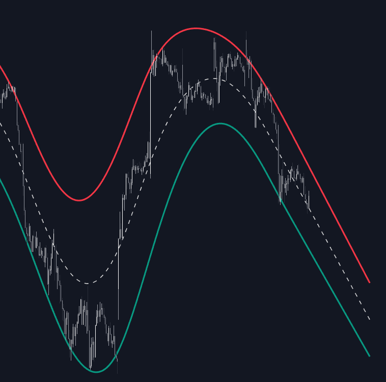
Two settings govern behavior. The difference order defines what smooth means: a second-order penalty pulls the fit toward a straight line as lambda grows, while a third-order penalty tolerates gentle curvature. Lambda then tunes the strength continuously: you trade fit for smoothness while the interior stays centered, rather than buying smoothness with ever more lag as a longer moving average would. For traders the appeal is a trend backbone clean enough to make slope, reversal points, and regime changes obvious; LuxAlgo's Whittaker Envelope builds its bands around exactly this curve.

How to apply and read a Whittaker–Henderson smoother

The smoother arrives as an indicator (the Whittaker Envelope is this library's implementation), and reading it well means respecting the split between settled interior and provisional end.

1Apply the indicator to closes and set the two controls: difference order (second or third) and penalty lambda, larger for smoother output.
2Tune lambda until the curve keeps the swings you care about and ignores the rest; an overlaid moving average of similar smoothness shows the lag saved by the global fit.
3Read trend from the interior: slope direction, steepness, and flattening are the signal, much as with an MA slope filter but with far less noise.
4Treat the newest bars as provisional: watch how much the fresh end revises on your settings before wiring any logic to it, and prefer confirmed structure for timing.

How it's calculated

The Whittaker-Henderson smoother is the series that minimizes a penalized least-squares objective, trading closeness to the data against smoothness of the output.

S(z) = \sum_{t=1}^{N} w_t \times (y_t - z_t)^2 + \lambda \times \sum_{t=d+1}^{N} (\Delta^d z_t)^2

z_1, \ldots, z_N = \text{the series minimizing } S(z)

\Delta^1 z_t = z_t - z_{t-1}

\Delta^2 z_t = z_t - 2 \times z_{t-1} + z_{t-2}

\text{Matrix form: } z = (W + \lambda \times D^T \times D)^{-1} \times W \times y

\text{With unit weights: } z = (I + \lambda \times D^T \times D)^{-1} \times y

t: bar index, 1..N

N: number of bars being smoothed

y_t: input value at bar t (typically the close); y is the input series as a vector

z_t: smoothed value at bar t; z is the output series as a vector (z_(t-1) and z_(t-2) are its prior values)

S(z): penalized least-squares objective, fit error plus roughness penalty

w_t: weight of bar t (default 1; 0 makes the smoother interpolate over that bar)

W: diagonal matrix holding the weights w_t

lambda: smoothness penalty, larger gives a smoother output (no universal default; tuned per series)

d: order of the penalized difference (default 2)

Δ^d z_t: d-th difference of z at bar t (lines 3 and 4 show d = 1 and d = 2)

D: (N - d) × N matrix form of the d-th difference operator; D^T is its transpose

I: N × N identity matrix

With d = 2 and unit weights this is the same construction as the Hodrick-Prescott filter; Whittaker's original 1923 graduation penalized third differences, and the method is also called the Whittaker or Whittaker-Eilers smoother.

lambda = 0 returns the input unchanged, and as lambda grows the output approaches a polynomial of degree d - 1 fitted to the window.

It is a whole-window, non-causal fit, so past values repaint as new bars arrive; the banded system solves in O(N).

How traders use it

As a trend curve for analysis: applied to closes it yields a smooth centerline whose slope and turning points are far easier to read than raw price, useful for assigning a trend regime label or studying past cycle turns.
As the basis of an envelope: offsetting the smoothed curve by a volatility measure builds an MA envelope-style band system around a very quiet centerline, read like other band systems, with the end-point caveat in mind.
As a pre-processing stage: feeding the graduated series into slope or momentum calculations cuts noise sharply, provided the workflow accounts for revisions at the fresh end of the window.
As a reference for real-time filters: traders tune a causal smoother such as an Ehlers SuperSmoother or an adaptive-lookback MA until it hugs the Whittaker curve acceptably, accepting some lag for values that never revise.

Whittaker–Henderson smoother vs other smoothing tools

SMA: An SMA is causal and equal-weighted: stable history, substantial lag, one length knob. Whittaker–Henderson fits the whole window at once, giving a centered, nearly lag-free interior at the cost of a revising end point.

EMA: An EMA reacts faster than an SMA but each value still depends only on the past, so it trails turns and never revises. The Whittaker curve turns almost with price in the interior, but its newest values are provisional.

Ehlers SuperSmoother: The SuperSmoother is a causal two-pole filter engineered to cut short-cycle noise with modest lag and no repainting, the closer real-time substitute when the Whittaker curve's revisions are unacceptable.

Concept family

Trend

100 concepts mapped · 100 in the Library

Whittaker–Henderson Smoother FAQ

Turn Whittaker–Henderson Smoother into a trading strategy.

Take the implementation from this page into Quant, then build on it, backtest it on real data, and keep refining it in conversation.

Previous conceptVWMA Next conceptWindowed FIR Smoothing