Correlation
Correlation, also known as Pearson, Spearman, rolling, correlation matrix, is a Statistics concept. The Library holds 9 implementations, each one a working definition you can pull into Quant.
Top Correlation indicators
The top custom implementations, built on the original standard Correlation formula.
9 total
Want to trade Correlation? Any of the 9 implementations below is one prompt away from a backtested strategy in Quant.
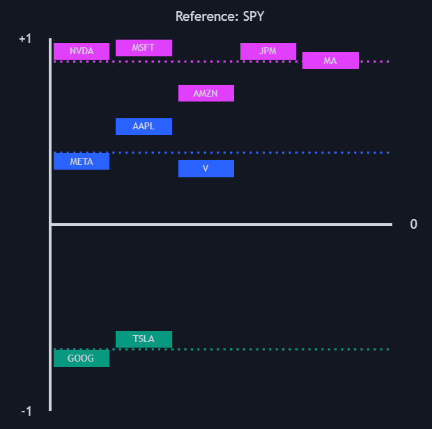
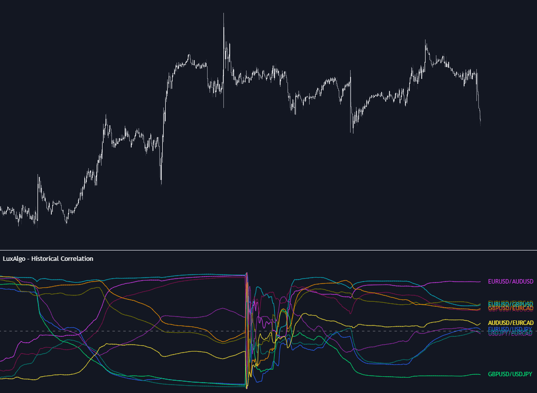
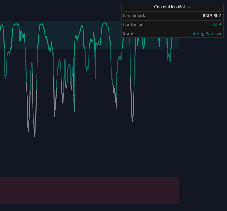
The standard Correlation indicator
Correlation exactly as classically defined: the faithful reference build of the original formula, free to run in Quant.
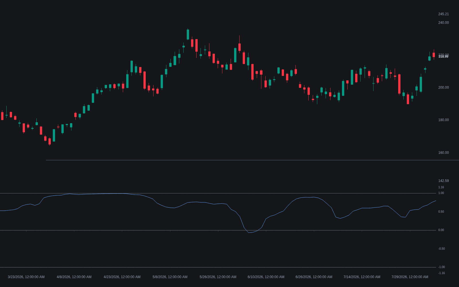
What is Correlation?
Correlation measures how consistently two series move together, on a scale from -1 to +1. The standard Pearson coefficient is the covariance of the two series divided by the product of their standard deviations: +1 means perfectly aligned moves, -1 perfectly opposite, 0 no linear relationship. The Spearman variant applies the same formula to ranks instead of raw values, which captures any monotonic relationship and blunts the effect of outliers. Traders usually compute it on returns over a rolling window, because raw trending prices produce inflated, spurious readings.
The mathematics predates its market use by decades. Francis Galton sketched the idea of co-relation in the 1880s while studying heredity, Karl Pearson formalized the product-moment coefficient in the 1890s, and Charles Spearman introduced the rank-based alternative in 1904. Quantitative finance adopted the machinery wholesale: Harry Markowitz's 1952 portfolio theory made the covariance matrix, and the correlations inside it, the central input to diversification, and essentially every risk model since has inherited both the tool and its assumptions.
It matters because almost every multi-asset decision hides a correlation assumption: positions that look diversified but move together behave like one oversized trade, intermarket filters assume yesterday's relationships persist, and relative-value trades need co-movement to lean on. The honest caveats: correlation is unstable over time, says nothing about cause, and describes direction of co-movement only, not size. It also tends to rise sharply across risk assets in stress episodes, precisely when diversification is needed most.
Correlation is also a windowed statistic: a 20-bar estimate reacts fast and whipsaws, a 200-bar estimate is stable but stale, so serious users watch more than one window or rank the current reading against its own history with a percentile rank. And Pearson's coefficient captures only linear dependence. Related tools pick up what it misses: linear regression turns the same relationship into slope and fit, autocorrelation applies the idea to a series' own past, and entropy measures attempt to detect dependence that has no linear shape at all.
How to calculate rolling correlation
Pearson correlation over a rolling window takes four steps, and the returns conversion in step one is the part that guards against spurious readings.
- 1Convert each series to returns or one-bar changes. Correlating raw prices overstates the relationship whenever both series trend, even if their day-to-day moves are unrelated.
- 2Choose a window N and, over the last N paired observations, compute each series' mean and its deviations from that mean.
- 3Multiply the paired deviations and sum them, then divide by the square root of the product of the two series' summed squared deviations. The result is the Pearson coefficient, bounded between -1 and +1.
- 4Plot the coefficient bar by bar as an oscillator. For Spearman correlation, replace the values in each window with their ranks first and apply the same arithmetic.
How it's calculated
Measures how tightly two series move together over a rolling window, from -1 (inverse) to +1 (lockstep).
Population and sample divisors (n vs n - 1) cancel in r, so both give the same coefficient.
The Spearman shortcut formula assumes no tied ranks; with ties, apply the Pearson formula to the ranks.
Rolling correlation recomputes r each bar; a correlation matrix computes the same r for every pair in a basket, and returns are often preferred over raw prices.
How traders use it
- As a portfolio exposure check: highly correlated positions stack the same risk, so correlation feeds position sizing and concentration limits rather than entry signals.
- As a directional filter: strategies condition entries on a driver series, for example trading a currency or index only when its rolling correlation with the dollar index or yields behaves the way the setup expects.
- As the first screen for relative value: pairs traders shortlist highly correlated instruments, then test cointegration separately, because two assets can be tightly correlated bar to bar while their spread drifts apart indefinitely.
- As a regime alarm: a rolling coefficient that collapses toward zero or flips sign flags that a historical relationship has broken, which matters most for hedges built on it.
- As an input to standardized spreads: once two instruments qualify, the spread between them is tracked as a z-score so that stretched has a definition; the correlation estimate justifies the pair, the z-score times the trade.
- For stress-testing assumptions: portfolio simulations such as Monte Carlo price paths embed a correlation matrix, and rerunning them with stressed correlations shows how much of a strategy's smoothness depends on relationships holding.
Correlation vs related concepts
Autocorrelation: Autocorrelation is a series correlated with its own past at some lag, a single-asset measure of persistence or mean reversion. Correlation as usually quoted compares two different instruments over the same bars.
Linear Regression: Correlation and regression are two views of the same fit: the coefficient measures how tight the linear relationship is, while regression estimates its slope and intercept, the numbers a hedge is built from. Correlation says the line fits; regression says what the line is.
Z-score: A z-score standardizes one series against its own mean and deviation; correlation compares two series. They meet in the formula: the Pearson coefficient is the average product of the two series' z-scores.
More Correlation implementations
Concept family
Statistics
46 concepts mapped · 46 in the Library
Correlation FAQ
Turn Correlation into a trading strategy.
Take any implementation from this page into Quant, then build on it, backtest it on real data, and keep refining it in conversation.