Is the Garman-Klass estimator more accurate than standard deviation of returns?

It is more statistically efficient under its assumptions (geometric Brownian motion, zero drift, no gaps), reaching a given precision with far fewer bars because the high-low range is informative. On real data the answer depends on how badly the assumptions fail: heavy overnight gapping or strong trend can bias it where close-to-close volatility is merely noisier.

Does the Garman-Klass estimator account for overnight gaps?

No. The classic formula sees only each bar's open, high, low, and close, so a jump from the prior close to the current open never enters it, and total volatility is understated on gap-prone assets. The Garman-Klass–Yang-Zhang hybrid adds the squared overnight return for exactly this reason, and the full Yang-Zhang estimator handles gaps and drift together.

What lookback window works best for the Garman-Klass estimator?

There is no single correct window. Because the estimator is efficient, short windows of 10 to 30 bars already give usable readings where close-to-close volatility would still be noisy. Shorter windows react faster but swing more; longer windows suit regime comparisons. Match the window to the decision it feeds and keep it consistent across instruments.

How is the Garman-Klass estimator annualized?

Average the per-bar variance over the window, multiply by the number of bars in a year, then take the square root. Daily data conventionally uses 252 trading days; intraday data uses bars per session times sessions per year. Tools differ in this constant, a common reason two platforms show different numbers from identical settings.

Can the Garman-Klass estimator replace ATR for stop placement?

It can, after conversion: de-annualize the volatility back to per-bar scale and multiply by price to get a distance. In practice many traders keep ATR for stops because it is already in price units and includes gaps, and use Garman-Klass where a statistically efficient annualized figure matters more.

Does the Garman-Klass estimator work on markets that trade around the clock?

Yes, and arguably best there. Continuous markets open where they closed, so the no-gap assumption approximately holds and the estimator's main blind spot disappears. The remaining caveats are drift bias during persistent trends and the slight underestimate of true extremes from discrete sampling in thin conditions.

Concept

Garman-Klass Estimator

Garman-Klass Estimator, also known as rolling Garman-Klass, is a Volatility concept. The Library holds 1 implementation, a working definition you can pull into Quant.

Top Garman-Klass Estimator indicator

The top custom implementation, built on the original standard Garman-Klass Estimator formula.

1 total

The Garman-Klass Estimator implementation below can become a backtested trading strategy — describe your rules and Quant writes the code.

Garman-Klass Estimator

Indicator

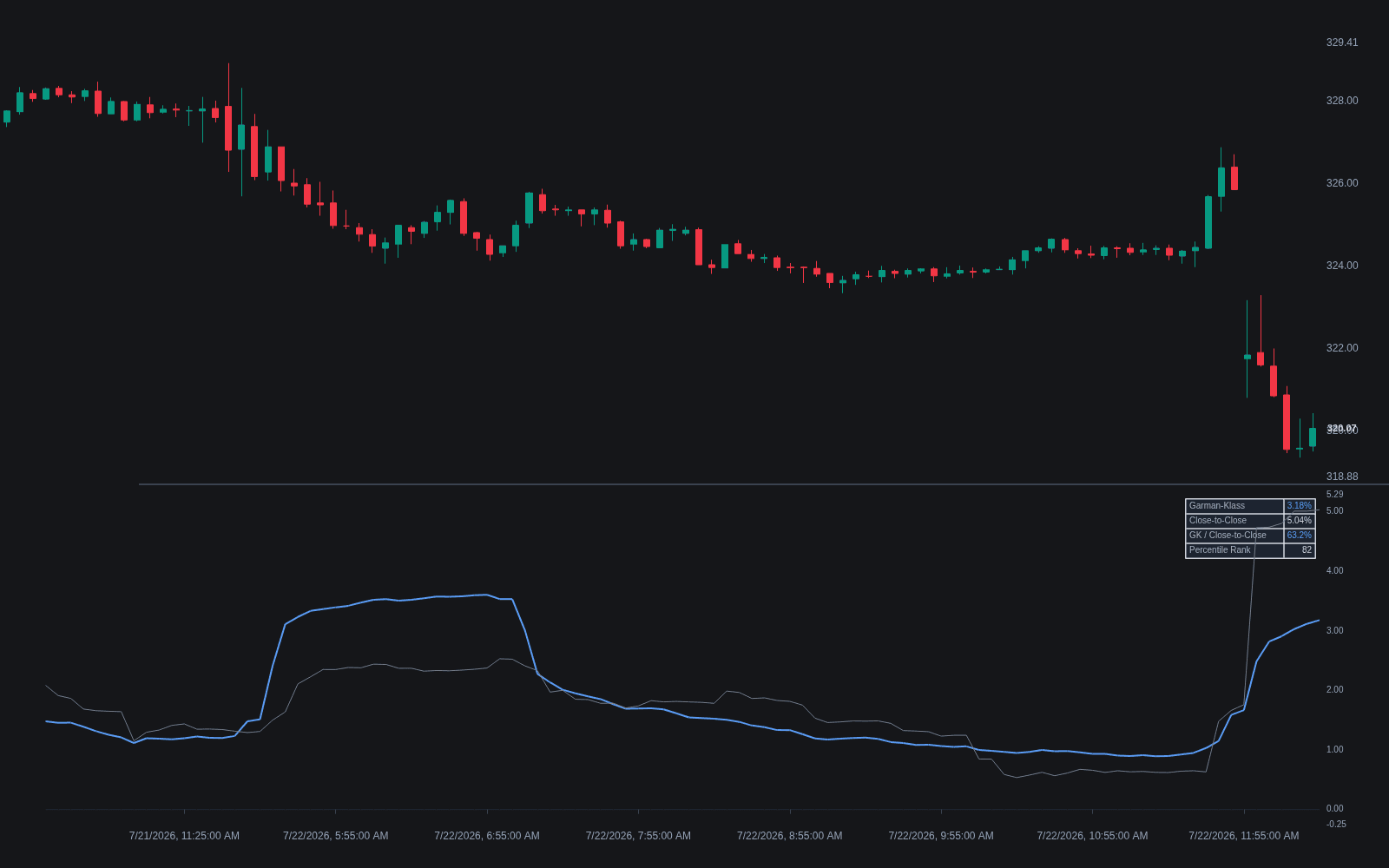
What is the Garman-Klass Estimator?

The Garman-Klass estimator computes historical volatility from each bar's open, high, low, and close rather than from closes alone. The per-bar variance estimate is half the squared log of high over low, minus (two times the natural log of two, minus one) times the squared log of close over open; averaging over a window and annualizing gives the volatility figure. Because the intrabar range samples the whole price path, the paper's theoretical efficiency gain over close-to-close realized volatility is roughly seven times under idealized assumptions.

The estimator comes from Mark Garman and Michael Klass, then at the University of California, Berkeley, whose paper On the Estimation of Security Price Volatilities from Historical Data appeared in the Journal of Business in 1980. It arrived alongside Michael Parkinson's high-low estimator the same year and improves on it by adding open-to-close information to the high-low term. Later authors patched its blind spots, but Garman-Klass remains the reference OHLC estimator the refinements are measured against.

Its assumptions are the catch: zero drift, continuous trading, and no opening gap. Anything that happens between one close and the next open is invisible to the formula, so gap-prone assets have their volatility understated. Strong trends violate the zero-drift assumption (the Rogers-Satchell estimator was built to fix exactly that), and discretely sampled highs and lows sit slightly inside the true extremes, which adds a small downward bias in thin or slowly traded markets.

The estimator matters because it changes what a volatility number is built from. ATR reacts to the same turbulence but is a smoothed range in price units, not a statistical variance estimate, and it cannot be annualized cleanly. Garman-Klass returns an annualized volatility comparable to options-style figures, which is why it appears as the width engine in band overlays and adaptive indicators, filling the role a standard deviation of closes plays inside Bollinger Bands with a steadier, range-aware reading.

How to identify the Garman-Klass estimator on a chart

The estimator is a computed series rather than a price pattern, so identification means recognizing its output and confirming which formula a tool actually implements.

1Add a Garman-Klass indicator, such as loxx's Garman & Klass Estimator Historical Volatility Bands; the output is either an annualized volatility line in a lower pane or bands drawn around price.
2Open the settings and note the lookback window and annualization factor; readings are typically annualized, so a daily estimate near 15 means roughly 15% annualized volatility.
3Plot a same-length close-to-close volatility beside it: the Garman-Klass line should track the same swells with visibly less bar-to-bar jitter, which is its efficiency signature.
4Watch a large overnight gap followed by a quiet session: the classic formula barely moves, confirming you are looking at gap-blind Garman-Klass rather than a gap-aware variant.
5Check that troughs in the series line up with visually compressed candles, the same stretches that BandWidth pinches or a TTM Squeeze flags.

How it's calculated

A range-based variance estimator that uses the whole OHLC bar, extracting more information per bar than close-to-close returns.

u_t = \ln\left(\frac{H_t}{L_t}\right)

c_t = \ln\left(\frac{C_t}{O_t}\right)

\operatorname{GK}_t = 0.5 \times u_t^2 - (2 \times \ln(2) - 1) \times c_t^2

\sigma^2 = \frac{1}{n} \times \sum_{t=1}^{n} \operatorname{GK}_t

\sigma = \sqrt{\sigma^2}

\text{Annualized:}\quad \sigma_{\text{ann}} = \sigma \times \sqrt{A}

O_t: open of bar t

H_t: high of bar t

L_t: low of bar t

C_t: close of bar t

t: bar index within the rolling window

ln(): natural logarithm

u_t: log high-low range of bar t

c_t: log open-to-close return of bar t

GK_t: single-bar variance estimate (the constant 2 × ln(2) - 1 ≈ 0.3863)

n: rolling window length in bars (commonly 10 to 30)

σ^2: Garman-Klass variance over the window

σ: Garman-Klass volatility per bar

σ_ann: annualized volatility

A: bars per year (252 for daily bars)

Derived by Garman and Klass (1980) assuming zero drift, continuous trading and no opening gaps; under those assumptions it is about 7.4 times as efficient as the close-to-close estimator.

Because overnight gaps are ignored it understates volatility for assets that jump between sessions; the Garman-Klass-Yang-Zhang variant adds a ln(O_t / C_{t-1}) gap term.

How traders use it

As a lower-noise volatility input: bands, stop distances, and sizing rules settle onto a stable reading with fewer bars, which matters when the lookback must stay short.
As a diagnostic pair with close-to-close volatility: Garman-Klass running well below it means movement is arriving as overnight gaps the formula cannot see; running above it means turbulent sessions whose closes mask the churn.
As one vote in an estimator composite, averaged with drift-robust and gap-aware alternatives so each covers the others' blind spots.
As a band width engine: de-annualized to per-bar scale and projected around a moving average, it builds envelopes that widen with statistical volatility, an alternative to ATR bands built on smoothed range.
As squeeze and regime context: ranking the series with a volatility percentile flags compressions that often precede expansion, a statistics-first complement to a Bollinger Squeeze read.

Garman-Klass vs other volatility measures

ATR: ATR averages true range in price units and includes gaps through the true-range definition, making it the natural stop-distance tool. Garman-Klass estimates annualized log-return variance, is gap-blind, and suits statistical uses such as volatility targeting or band width.

Realized Volatility: Standard realized volatility squares close-to-close returns, so it sees gaps but wastes the intrabar path and needs long windows to stabilize. Garman-Klass extracts more from each bar via the open-high-low-close geometry, at the cost of missing overnight moves.

BandWidth: BandWidth reads volatility indirectly as the spread of Bollinger Bands, a rescaled standard deviation of closes. Garman-Klass is a direct OHLC variance estimator independent of any overlay, and the two can disagree when gaps or intrabar churn dominate.

Concept family

Volatility

57 concepts mapped · 57 in the Library