Inverse Fisher Transform

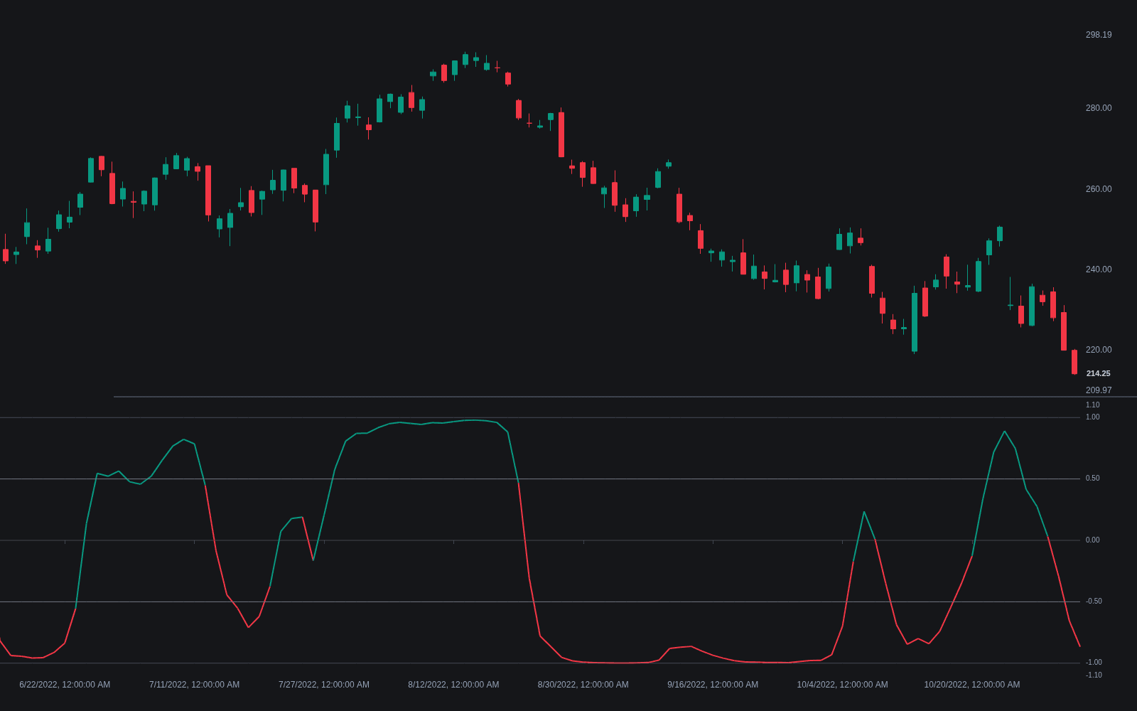
What is the Inverse Fisher Transform?

The Inverse Fisher Transform is John Ehlers' recipe for making an oscillator's output more decisive. It runs a zero-centered input through (e^(2x) - 1) / (e^(2x) + 1), which is algebraically the hyperbolic tangent: an S-curve that compresses everything into -1 to +1. The curve is nearly linear for small inputs, but moderately strong inputs get pushed hard toward the rails, so with the input scaled sensibly the transformed oscillator spends most of its time saturated near an extreme and crosses the middle quickly.

Ehlers, an engineer who spent his career porting digital signal processing into market analysis, published the technique in a 2004 Technical Analysis of Stocks & Commodities article. His aim was practical: oscillators spend too much of their life in ambiguous mid-range territory, leaving the trader to guess. Reshaping the output so it is clearly high, clearly low, or briefly in transit turns the same information into something closer to a switch.

Ehlers' published example applied it to RSI: center a short RSI on zero, scale it down, smooth it with a weighted moving average, then transform, with crossings of ±0.5 as the conventional triggers. It is the counterpart of the Fisher Transform, which stretches tails to sharpen extremes; the inverse compresses them to create clean, nearly binary states.

Implementation is mostly a scaling exercise. Ehlers' example took a 5-period RSI, subtracted 50, multiplied by 0.1 so typical values land in the curve's active region, and smoothed with a 9-period weighted moving average before transforming. The caveats follow from the design: smoothing adds a little lag, and in a persistent trend the output saturates on one side for long stretches, so a +1 reading is a regime label rather than an overbought sell signal. The same treatment fits any zero-centered input, from a scaled CCI to stochastic variants.

How to read an Inverse Fisher Transform oscillator

The plot is a bounded line hugging ±1 with fast transitions; reading it means knowing the pipeline behind it.

1. 1Know the pipeline: a base oscillator (a 5-period RSI is the classic), centered on zero, scaled, smoothed, then transformed. Different inputs produce differently behaved lines.
2. 2Mark the ±0.5 levels: the cross up through -0.5 is the conventional buy trigger and the cross down through +0.5 the conventional sell or exit.
3. 3Read saturation as state: a line pinned near +1 marks a persistent bullish regime, not an automatic fade; the same holds near -1.
4. 4Watch dwell time in the middle: quick transits are the design working, while hovering around zero flags a choppy market where the transform whipsaws.
5. 5Check the scale factor before comparing charts: it controls how often the rails are reached, so two implementations can disagree on the same data.

How traders use it

• As a signal cleaner: applied to RSI, stochastics, or the Stochastic Momentum Index, it converts fuzzy overbought/oversold territory into saturated states, with the cross up through -0.5 and down through +0.5 as the standard triggers.
• As a compact regime flag: because the output sits near +1 or -1 most of the time, it summarizes an oscillator's state cleanly for dashboards, screeners, and multi-timeframe panels.
• As a normalization stage: it is one of the sigmoid-style transforms used to squash inputs into a fixed range before combining or thresholding signals.
• As exit management: positions are held while the transform stays saturated and closed when it crosses back through the ±0.5 boundary, letting the S-curve define when momentum is spent.
• With a trend filter: because the output can sit saturated against a trend for long stretches, many traders pair it with MACD or moving-average slope and take only crossings that agree with it.

Inverse Fisher Transform vs related oscillators