What does the Fisher Transform actually do to price?

It rescales price (usually the bar midpoint) into a -1 to +1 range over a lookback window, then applies half the natural log of the ratio (1 + x) / (1 - x). That reshapes the value distribution toward a Gaussian: middling readings stay small while near-extreme readings are stretched dramatically, so tops and bottoms print as sharp, isolated peaks instead of rounded plateaus.

Is the Fisher Transform a leading indicator?

It is fast rather than prophetic. Because the transform sharpens extremes and uses minimal smoothing, its turns often print a bar or two before heavily smoothed oscillators. It still cannot anticipate anything: in choppy conditions the same speed produces frequent whipsaw crossovers, so most users pair it with a trend or volatility filter and accept that early signals fail regularly.

Where does the Fisher Transform formula come from?

From classical statistics. Fisher's z-transformation was devised to make the distribution of correlation coefficients approximately normal so standard inference could apply, and Ehlers borrowed the identical function for price in his 2002 article. The repurposing works because the problem is the same shape: a bounded quantity whose interesting behavior happens near its limits, exactly where its raw distribution is most distorted.

What lookback should the Fisher Transform use?

Ehlers' original used 10 bars for the normalization window, and it remains the default. Shorter windows make the normalization twitchier, so extremes arrive more often and mean less; longer windows slow the indicator toward ordinary oscillator behavior and blunt the sharp turns that justify the transform. The window is really defining what counts as an extreme, so it should match the swing size you intend to trade.

Why is the input capped just inside ±1?

Because the transform has singularities at exactly ±1: the log ratio goes to infinity as x approaches either limit. Implementations clamp the normalized input around ±0.999 so the output stays finite while preserving the stretched-tail behavior. The cap is a numerical guard, not a tuning parameter, though it does set the maximum value the indicator can print.

Can the Fisher Transform be applied to other indicators?

Yes, and Ehlers encouraged it: any bounded or normalizable series can be pushed through the same function to sharpen its turning points, which is how Fisher-transformed stochastics and similar hybrids arise. The requirements are just the preprocessing, rescale the series into ±1 over a window and cap it, and the same reading rules: crossings after extremes matter, mid-range crossings are noise.

Concept

Fisher Transform

Fisher Transform is a Momentum & Oscillators concept. The Library holds 1 implementation, a working definition you can pull into Quant.

The standard Fisher Transform indicator

Fisher Transform exactly as classically defined: the faithful reference build of the original formula, free to run in Quant.

Fisher Transform

Indicator

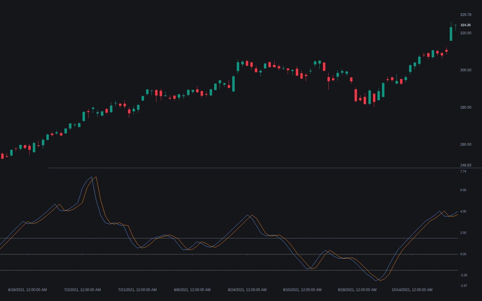
What is the Fisher Transform?

The Fisher Transform is John Ehlers' technique for reshaping price data into an approximately Gaussian (normal) distribution. It first rescales price, typically the bar midpoint, into a -1 to +1 range over a short lookback window (10 bars in Ehlers' original article), a smoothed form of min-max scaling, then applies the transform: half the natural logarithm of the ratio (1 + x) / (1 - x), with the input capped just inside ±1 so the logarithm stays finite. The effect is to stretch the tails: mid-range readings stay small, while readings near the extremes expand into sharp, isolated peaks.

Ehlers' argument was that price is not normally distributed, so turning points in ordinary oscillators come out rounded and mushy. After the transform, extreme values are rare and reversals show up as sharp slope changes. The standard signal set reflects that: the Fisher line crossing its own one-bar-delayed copy, plus extreme absolute readings marking stretched conditions, rather than fixed overbought/oversold lines.

The mathematics is borrowed, not invented: Fisher's z-transformation is a classical statistics tool for making correlation coefficients approximately normal, and Ehlers repurposed it for prices in his 2002 Technical Analysis of Stocks & Commodities article. The Gaussian reshaping is what gives the extremes their meaning. On a roughly normal output, readings beyond about two are genuinely rare events rather than routine visits to the rail, so a spike and hook in that territory carries statistical weight that a bounded oscillator pinned at 100 cannot claim. The sharpness serves the same end: because the tails are stretched, the slope change at a turn is violent and unambiguous rather than a rounded drift.

The transform travels well beyond its own indicator. Applied to a stochastic or any bounded series, it sharpens that tool's turns the same way, which is why it appears as a preprocessing stage across the Ehlers-influenced toolkit; hybrid builds like the SuperTrend Fisher run regime logic on transformed values, and least-squares variants swap the input smoothing. Its mirror image, the Inverse Fisher Transform, compresses instead of stretches, pushing an oscillator toward binary extremes. The standing caveat is speed's usual bill: minimal smoothing plus sharpened extremes means frequent whipsaw crossings in chop, so the classic deployment pairs it with a trend or volatility filter.

How to identify the Fisher Transform

Two stages, one signal convention: normalize, transform, then read the crossings.

1Take the bar midpoint (high plus low, halved) and rescale it into -1 to +1 over the lookback, 10 bars in the original, with light smoothing on the scaled value.
2Cap the scaled input just inside ±1, conventionally ±0.999, so the logarithm cannot blow up.
3Apply the transform: half the natural log of (1 + x) divided by (1 - x), usually with a touch of smoothing on the output.
4Plot the signal line: the Fisher value delayed one bar, so crossings of the pair mark slope changes.
5Read it Ehlers' way: crossings that occur after an extreme absolute reading are the primary events; crossings in the mid-range are chop by construction.

How it's calculated

The Fisher Transform maps where price sits inside its recent range through the inverse hyperbolic tangent, producing an oscillator whose distribution is close to Gaussian with sharp turning points.

P_t = \frac{H_t + L_t}{2}

X_t = 0.66 \times \left(\frac{P_t - \operatorname{MinP}_n}{\operatorname{MaxP}_n - \operatorname{MinP}_n} - 0.5\right) + 0.67 \times X_{t-1}

\text{If } X_t > 0.99 \text{ set } X_t = 0.999\text{; if } X_t < -0.99 \text{ set } X_t = -0.999

\operatorname{Fisher}_t = 0.5 \times \ln\left(\frac{1 + X_t}{1 - X_t}\right) + 0.5 \times \operatorname{Fisher}_{t-1}

\operatorname{Trigger}_t = \operatorname{Fisher}_{t-1}

H_t: high of bar t

L_t: low of bar t

t: bar index

P_t: median price of bar t

MinP_n: lowest P over the last n bars

MaxP_n: highest P over the last n bars

n: lookback length (commonly 9 or 10)

X_t: smoothed position of price inside its range, held between -1 and +1 (X_{t-1} is the prior value)

ln(): natural logarithm

Fisher_t: Fisher Transform value at bar t (Fisher_{t-1} is the prior value)

Trigger_t: signal line, the Fisher value delayed one bar

0.5 × ln((1 + X_t) / (1 - X_t)) is the inverse hyperbolic tangent of X_t; the clamp keeps it finite when price pins the top or bottom of the range.

The 0.66 and 0.67 constants are John Ehlers' fixed smoothing of the range position; his original length is 10, and many platforms default to 9.

How traders use it

As a turn timer: the classic trigger is the Fisher line crossing its one-bar-delayed signal line after an extreme reading, which tends to print earlier (and more often) than signals from heavily smoothed oscillators.
As a stretch detector: because the transformed values are approximately Gaussian, large absolute readings are statistically unusual, so traders treat them as zones to tighten stops, take profits, or watch for reversal, not as automatic fades.
As a preprocessing step: the same transform is applied to other oscillators to sharpen their turns, while its counterpart, the Inverse Fisher Transform, does the opposite job and compresses an oscillator toward binary extremes.
In hybrid regime tools: builds like SuperTrend Fisher feed transformed values into stop-and-reverse logic, borrowing the transform's sharp extremes to make regime flips more decisive.
With a filter in front: because speed is the design, most deployments gate Fisher signals with a trend or volatility condition, taking the with-trend crossings and ignoring the counter-trend chatter the transform's sensitivity produces.

Fisher Transform vs related oscillators

Stochastic Oscillator: Both begin from range-relative position, but the stochastic stays bounded and rounds off at its rails, while the Fisher stretches those extremes into sharp Gaussian tails. The stochastic asks where price sits in its range; the Fisher asks how statistically unusual that position is.

Inverse Fisher Transform: Exact opposites in intent: the Fisher expands the tails so turns print sharply, the inverse compresses everything toward ±1 so an oscillator becomes almost binary. One is built for timing turns, the other for clean regime reads with suppressed mid-range noise.

RSI: RSI reshapes price through gain-loss averaging and lives on a bounded scale that saturates in strong trends. The Fisher reshapes the distribution itself, keeping extremes rare and meaningful. RSI's strength is its conventions; the Fisher's is the statistical honesty of its extremes.

Concept family

Momentum & Oscillators

91 concepts mapped · 91 in the Library

Fisher Transform FAQ

Turn Fisher Transform into a trading strategy.

Take the implementation from this page into Quant, then build on it, backtest it on real data, and keep refining it in conversation.

Previous conceptFirefly Oscillator Next conceptGator Oscillator